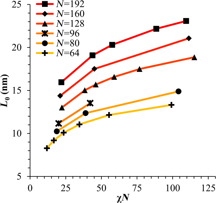
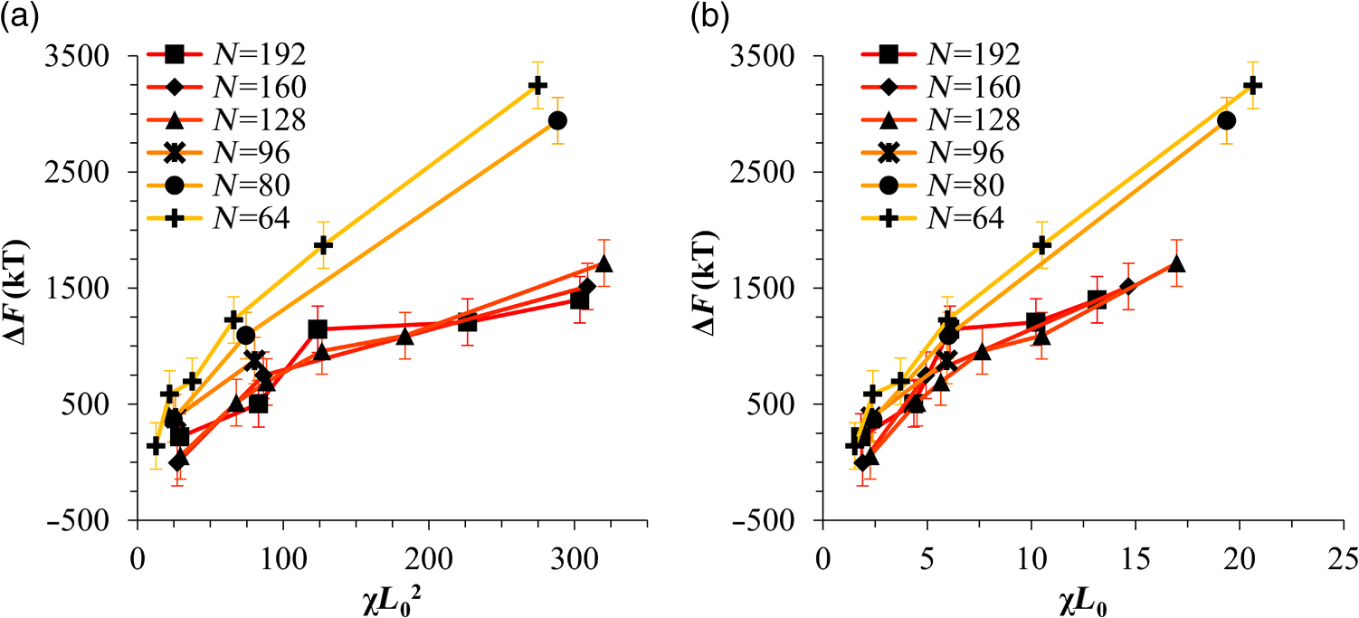
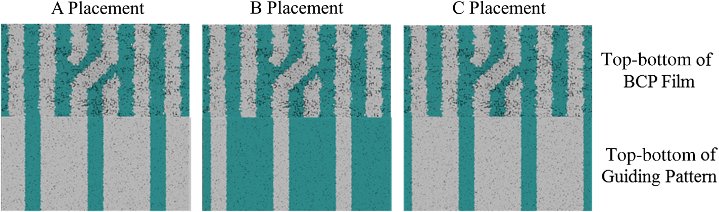
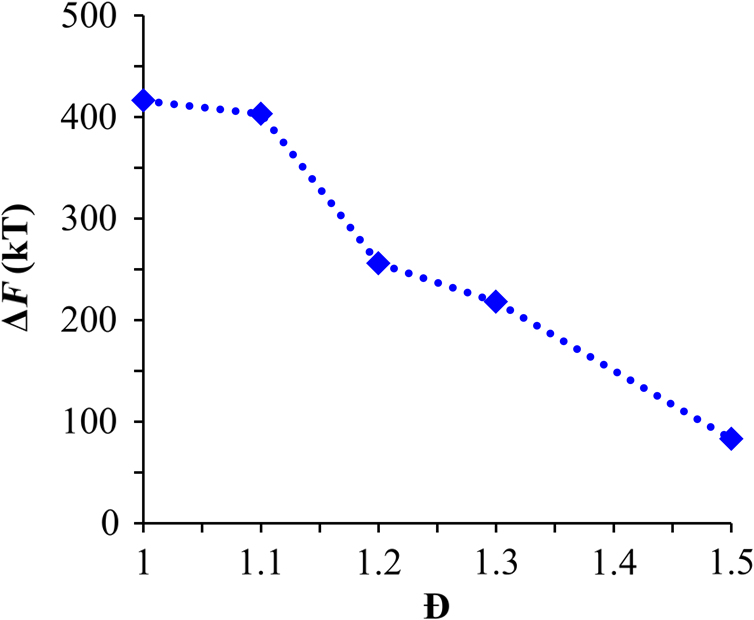
1.

Introduction

Block copolymer (BCP) directed self-assembly (DSA) is a technique that has been studied extensively in recent years for use in nanofabrication because it excels in rapidly producing nanoscale patterns with long-range order when aligned to a prepatterned underlayer.^1,2 The most common methods to align such BCPs include using a chemically patterned underlayer,³ a topographically patterned underlayer,⁴ or some combination of the two.^5,6 Such techniques are being engineered to be more capable of producing useful patterns including aligned lamellae and cylinder phases that mimic the types of patterns useful in semiconductor device fabrication, but many obstacles still exist to their practical use industrially. One of the most critical obstacles is that of defect density. Progress has been made toward understanding the fundamental cause of these defects,^7–9 including the calculation of the defect free energy ($\mathrm{\Delta }F$) using a self-consistent field theory model in laterally confined systems⁷ and how this free energy changes as a function of guiding linewidth.⁷ In the context of such laterally confined systems, the effect of molar mass dispersity ($\mathit{Ð}$) was studied,⁷ but only for binary blends, which is a poor model for the dispersity inherent in a typical BCP system. Work using a coarse-grained model has studied the effect of pattern-guiding strength on a $1:1$ pattern.⁸ However, current defect concentrations are orders of magnitude above necessary levels for many microelectronic applications^10,11 and the effects of numerous variables, including $\chi$ (the Flory Huggins interaction parameter), $\chi N$ (where $N$ is the degree of polymerization), and various guiding layer properties on defect formation are still not understood.

The study of these DSA problems can be aided greatly by the use of computer simulations, particularly in the area of defect modeling. Differentiating guiding pattern effects from inherent BCP defects and from particle or other contaminating factors is very difficult experimentally. Furthermore, the identification of the equilibrium defectivity and separating that from kinetic aspects of defect formation and annihilation is difficult, but crucial to understanding BCP defects and removing them in BCP-DSA processes. Simulations can much more easily achieve these goals. By using thermodynamic integration, coarse-grained molecular dynamics simulations can provide calculation of the free energy difference between two states, although a reversible path between them must be formulated. The free energy of a defect can be calculated as a function of various polymer and underlayer properties to provide insight into what property variations might minimize the occurrence of defects. This insight can then be applied to focus experimental investigations.

This work will study one of the most common defects found in BCP-DSA processes, a dislocation pair, or jog defect. This defect is shown in Fig. 1 and has been observed in various experiments^7–9,12,13 and in our own simulations. A dislocation pair (a dislocation is the “Y” structure in cyan in Fig. 1) can be separated by different numbers of lamellae, but this work will study a defect separated by a single domain, which is quite commonly seen in BCP-DSA.

Fig. 1

Top bottom image of the defect type studied in this paper. This is a common defect found in the literature.^7–9,12,13 The $A$ beads are shown in white, while the $B$ beads are shown in cyan.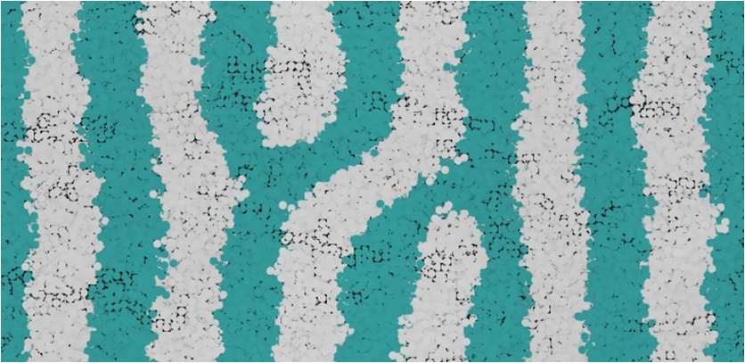

While such defects occur for various pattern types and various polymers, a good understanding of how these patterns and polymer properties actually affect defect density is lacking. The defect density ($n_{\mathrm{d}}$) can be described as

2.

Models and Methods

2.1.

Coarse-Grained Model

A coarse-grained polymer model has been used and is described in detail elsewhere,^16,17 but a brief description will be given here. Molecules are coarse-grained by modeling four monomeric units as a single bead. Four monomers were chosen because this approximately corresponds to the statistical segment length of polystyrene and poly(methyl methacrylate), two common polymers studied in BCP DSA. Beads were connected using harmonic potentials. A harmonic angle potential was also used between every set of three consecutively bonded beads to prevent collapse due to nonbonded interactions. Every pair of beads that does not participate in the same angle potential (i.e., every bead that is on a different molecule or that is more than two bonds away) interact via a nonbonded potential similar to a Lennard–Jones potential as

Eq. (2)

$$E_{\text{Nonbonded}}={ϵ}_{ij}[{\left(\frac{{\sigma }_{ij}}{r}\right)}^8-2{\left(\frac{{\sigma }_{ij}}{r}\right)}^4].$$

The parameter ${ϵ}_{ij}$ is the depth of the potential well, which corresponds to the strength of the interaction and to cohesive energy density. ${\sigma }_{ij}$ is the location of the minimum of the potential, which controls the average spacing between noncovalently bonded beads and the density of the system. The exponents in Eq. (2) are lower than in the Lennard–Jones potential expression because these fit the coarse grain potential well and reflect the averaging effect of the coarse-grained potential. In this work, the parameters for both $A$ and $B$ blocks are chosen to roughly reproduce the density and segment distribution of polystyrene. ${ϵ}_{AA}$ and ${ϵ}_{BB}$ are set to $0.5\mathrm{kcal}/\mathrm{mol}$, while ${\sigma }_{AA}$, ${\sigma }_{BB}$, and ${\sigma }_{AB}$ are set to 1.26 nm. The equilibrium bond length used for both $A$ and $B$ polymers was 0.82 nm with a harmonic strength of $100\mathrm{kcal}/\mathrm{mol}·{\mathrm{nm}}^2$. The equilibrium angle used for both $A$ and $B$ polymers was $2\pi /3$ radians (120 deg) with a harmonic strength of $5\mathrm{kcal}/\mathrm{mol}·{\text{radian}}^2$. Simulations were run at 500 K, a realistic thermal anneal temperature for DSA-BCP systems, with a time step of 0.05 ps. Further discussion of these parameters can be found elsewhere.^16,18,19 Because ${ϵ}_{AB}$ describes the interaction between unlike blocks, this parameter is used to determine the value of the Flory–Huggins enthalpic interaction parameter $\chi$. To determine $\chi$, we fit the structure factor (a component of the x-ray diffraction profile) to Leibler’s theory for BCP scattering similar to its extraction from the experimental results.^20,21 The ${ϵ}_{AB}-\chi$ relation is extrapolated from this fit in the mixed state to lower ${ϵ}_{AB}$ values. This gives a relation for $\chi$ as a function of ${ϵ}_{\mathrm{AB}}$, $N$, and volume fraction of the $A$ block which is important in understanding our results relative to other calculations that primarily describe their potentials with the $\chi$ parameter. Details of this method can be found elsewhere.²² Justification for the linear extrapolation follows: $\chi$ is defined by Flory²³

Eq. (3)

$$\chi =z\mathrm{\Delta }w/kT,$$

where $z$ is the coordination number, $\mathrm{\Delta }w$ is the exchange energy, $k$ is the Boltzmann constant, and $T$ is the temperature of the system. The exchange energy, $\mathrm{\Delta }w$, is defined as the energy penalty for replacing an $A-A$ or a $B-B$ interaction with an $A-B$ interaction

Eq. (4)

$$\mathrm{\Delta }w=w_{\mathrm{AB}}-\frac{1}{2}(w_{\mathrm{AA}}+w_{\mathrm{BB}}),$$

where $w_{\mathrm{AB}}$ is the interaction energy between an $A$ bead and a $B$ bead. Since the interaction energy in this model is defined by the nonbonded potential parameter $ϵ$, $\mathrm{\Delta }w$ can be defined for our system as

Eq. (5)

$$\mathrm{\Delta }w={ϵ}_{\mathrm{AB}}-\frac{1}{2}({ϵ}_{\mathrm{AA}}+{ϵ}_{\mathrm{BB}}).$$

This shows that $\mathrm{\Delta }w$ scales linearly with changes in ${ϵ}_{\mathrm{AB}}$. As long as the density of the $A-B$ interface does not significantly perturb the system, $z$, the coordination number (the number of beads a single bead interacts with), will remain a constant. Since $kT$ is a constant, $\chi$ will scale linearly with ${ϵ}_{\mathrm{AB}}$ until $z$ is perturbed by density variations at the $A-B$ interface. All simulations were run using the HOOMD-Blue software package^24,25 and visualized in VMD.²⁶ The natural parallelizability of MD simulations and the GPU optimization of HOOMD allows simulations on a GPU enabled computer to run up to 200 times faster than a desktop computer (Intel Core 2 Duo $\sim 2\mathrm{GHz}$, 2GB RAM).

The natural repeat distance $L_0$ of each set of $\chi$ and $N$ is measured using the structure factor, which provides similar information to that of a scattering experiment.^22,27 The values of $L_0$ used here are shown in Fig. 2.

Fig. 2

Plot of $L_0$ dimensions as used in this work. Dimensions were measured using the structure factor.^22,27

2.2.

Thermodynamic Integration

A method similar to that used by de Pablo and coworkers⁸ and Müeller and coworkers²⁸ was used to determine free energy changes. The free energy difference between two states can be calculated as

Eq. (6)

$$\mathrm{\Delta }{F}_{a\to b}=\underset{u_A}{\overset{u_B}{\int }}\langle \frac{\delta H}{\delta u}\rangle \mathrm{d}u.$$

$H$ is the classical Hamiltonian of our model, $u$ is any parameter that when varied defines a continuous, thermodynamically reversible path between state $A$ and state $B$, and the brackets $\langle ·\rangle$; denote a thermodynamic average, that is the average value at equilibrium. The states used were a dislocation pair or jog defect (Fig. 1) and a defect free ordered lamellae state. Instead of trying to define a reversible, continuous path between a well-aligned lamellar state and a defect free state, it is easier for our model to use two different paths, i.e., a path from a mixed state to a lamellar state and a path from a mixed state to a defective state. Therefore in order to compare the defective and defect free states, two simulations were run as described in Fig. 3: one from a mixed state to a defect free lamellae state, which yields the free energy difference between the mixed state and the defect free state ($\mathrm{\Delta }{F}_{\text{DefectFree}-\text{Mixed}}$), and another simulation from a mixed state to a defective state, which yields the free energy difference between a mixed state and a defective state ($\mathrm{\Delta }{F}_{\text{Defect}-\text{Mixed}}$). Then

Eq. (7)

$$\mathrm{\Delta }{F}_{\text{Defect}-\text{DefectFree}}=\mathrm{\Delta }{F}_{\text{Defect}-\text{Mixed}}-\mathrm{\Delta }{F}_{\text{DefectFree}-\text{Mixed}}.$$

Both $\mathrm{\Delta }{F}_{\text{Defect}-\text{Mixed}}$ and $\mathrm{\Delta }{F}_{\text{Defect}-\text{Free}-\text{Mixed}}$ were calculated using three branches of the MD simulation. The first branch is used to order the mixed polymers into the desired morphology. This was done using an external potential, which assigns an energy to beads based on their type and position within the simulation. In the case of the defect free state, the external potential energy was described as

Eq. (8)

$$U_{\mathrm{def}-\text{free}}=A\tanh \left[\frac{\cos \left(\frac{2\pi x}{L}\right)}{2\pi w}\right],$$

where $A$ is the strength of the potential, $x$ is the position in the $x$ axis of the bead, $w$ is the width of the interface of the potential, and $L$ is the repeat distance of the potential. The defect potential is created using the same equation, except the center portion is rotated 45 deg.

Eq. (9)

$$U_{\mathrm{def}}=\{\begin{array}{ll}{U}_{\text{in}}& -0.75L_0<x<0.75L_0\\ & -0.5L_0<y<0.5L_0\\ U_{\text{out}}& \text{otherwise}\end{array},$$

Eq. (10)

$$U_{\text{in}}=A\tanh \left(\frac{\cos \left\{\frac{2\pi [x\cos (\pi /4)-y\sin (\pi /4)]}{L_0}\right\}}{2\pi w}\right),$$

Eq. (11)

$$U_{\text{out}}=A\tanh \left[\frac{\cos \left(\frac{2\pi x}{L_0}\right)}{2\pi w}\right].$$

Fig. 3

Schematic of the method used to calculate the defect free energy. Two simulations are run: one from the mixed to the defective lamellar state and one from the mixed to the defect free lamellar state. Each of these simulations yields the free energy difference between the mixed state and the corresponding final state. The difference between the two free energies is the free energy difference between the defect and the defect free state. Each simulation contains three branches over which a free energy difference is calculated. The first branch orders the system from the mixed state using an external potential, the second changes $\chi$, and the third turns off the external potential.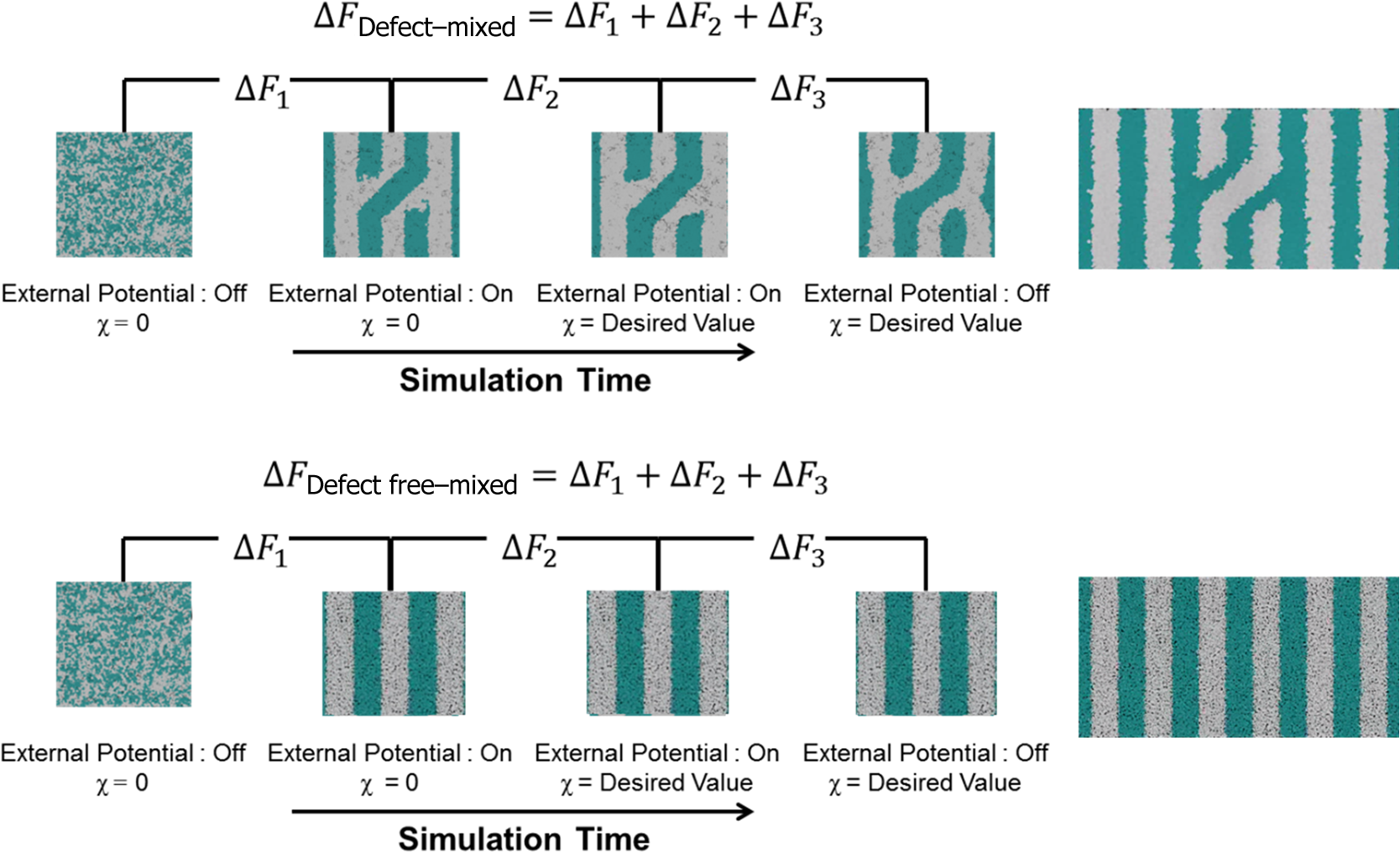

This produces the dislocation pair defect found in both our simulations and in published experimental results.^7–9,12,13 The integral from Eq. (6) was carried out where the reversible path ($u$) is defined by changes in the strength of the external potential, $A$. This integral, which yields $\mathrm{\Delta }{F}_1$ from Fig. 3, is shown in Eqs. (12) and (13) for the defect free case.

Eq. (12)

$$\mathrm{\Delta }{F}_1=\underset{0}{\overset{A_{\max }}{\int }}\langle \frac{\delta U_{\mathrm{def}-\text{free}}}{\delta A}\rangle \mathrm{d}A=\underset{0}{\overset{A_{\max }}{\int }}\langle \frac{U_{\mathrm{def}-\text{free}}}{A}\rangle \mathrm{d}A,$$

Eq. (13)

$$\mathrm{\Delta }{F}_1=\underset{0}{\overset{A_{\max }}{\int }}\langle \tanh \left[\frac{\cos \left(\frac{2\pi x}{L_0}\right)}{2\pi w}\right]\rangle \mathrm{d}A,$$

where $A_{\text{max}}$ is 2.6. The defective case is identical except that $U_{\mathrm{def}}$ is substituted for $U_{\mathrm{def}-\text{free}}$.

The integrals [Eqs. (12) and (13)] were evaluated by numerically increasing $A$ in 100 fixed-increment steps from 0 to $A_{\text{max}}$, which in this case was 2.6. At each step, an MD simulation is run at the new value of $A$ until the simulation has equilibrated, and the average value at equilibrium is taken and used in integrating Eq. (13). In order to confirm the amount of time required to run the simulation at each step in the ramp up of $A$, multiple simulations were run for various lengths and the free energy integration was performed, as shown in Fig. 4. Short times showed significant deviations from the results at long times, because a short integration time does not allow the system sufficient time to equilibrate, making the path irreversible. At long times, the simulations are able to reach equilibrium at each step, and therefore the path is reversible and the measured free energy approaches a constant value. A value of 320,000 time steps per step in $A$ was found to be sufficient and therefore was chosen to be used for the remainder of the paper. In Fig. 4 initially the value of the integrand is close to zero while the system is not well ordered. As the system phase separates due to the increasing strength of the external potential, the value of the integrand begins to approach a constant value. Figure 4 shows a sharp bend at $A\sim 0.4$. At this point, the system is mostly already phase separated, and the remainder of the simulation primarily consists of decreasing the interfacial roughness of the BCP.

Fig. 4

Plot of the integrand of Eq. (13) as $A$ is increased. As the number of timesteps per step in $A$ is increased, the curves converge. A value of 320,000 was used to ensure accuracy and reasonable simulation times.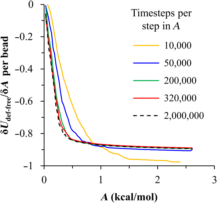

Once the BCP has been ordered in the first branch of the simulation, $\chi$ (which was initially kept at zero during the first branch by setting ${ϵ}_{AB}={ϵ}_{AA}={ϵ}_{BB}$) must be increased. The starting condition had a $\chi$ of 0 so that the initial equilibrium state of the system was a well-defined, well-mixed state. In our model, $\chi$ is controlled by changing only ${ϵ}_{AB}$, so ${ϵ}_{AB}$ was varied from $0.5\mathrm{kcal}/\mathrm{mol}$ ($\chi =0$) to whatever value was desired, allowing the defect free energy to be calculated as a function of $\chi$. Equation (6) was then integrated where $u$ is now ${ϵ}_{AB}$, resulting in Eq. (14). This results in $\mathrm{\Delta }{F}_2$ from Fig. 3.

Eq. (14)

$$\mathrm{\Delta }{F}_2=\underset{0.5}{\overset{{ϵ}_{AB\_\text{Final}}}{\int }}\langle \frac{\delta U_{\text{nonbonded}}}{\delta {ϵ}_{AB}}\rangle \mathrm{d}{ϵ}_{AB}=\underset{0.5}{\overset{{ϵ}_{{AB}_{\text{Final}}}}{\int }}\langle \frac{U_{\text{nonbonded}}}{{ϵ}_{AB}}\rangle \mathrm{d}{ϵ}_{AB},$$

Eq. (15)

$$\mathrm{\Delta }{F}_2=\underset{0.5}{\overset{{ϵ}_{AB\_\text{Final}}}{\int }}[{\left(\frac{{\sigma }_{AB}}{r}\right)}^8-2{\left(\frac{{\sigma }_{AB}}{r}\right)}^4]\delta {ϵ}_{AB}.$$

$U_{\text{nonbonded}}$ is used because $\chi$ is changed via ${ϵ}_{AB}$ and the nonbonded potential is the portion of the Hamiltonian in which ${ϵ}_{AB}$ appears. The value ${ϵ}_{AB\_\text{Final}}$ is the value of ${ϵ}_{AB}$ that yields the desired $\chi$. This value will be less than the value of ${ϵ}_{AB}=0.5$, which yields $\chi =0$. The number of time steps per step in ${ϵ}_{AB}$ was varied and the integrand measured as for branch 1. The results are found in Fig. 5. In this case, even very low numbers of timesteps per step in ${ϵ}_{AB}$ yield the same result as very long runs. This is because there is little to no overall morphological change in this branch as there was in branch 1. This integration was done in 50 steps and run for 40,000 ps for each step in ${ϵ}_{AB}$.

Fig. 5

Plot of the integrand of Eqs. (14) and (15) as ${ϵ}_{AB}$ is increased. All values of time steps per step in ${ϵ}_{AB}$ yield the same integrand.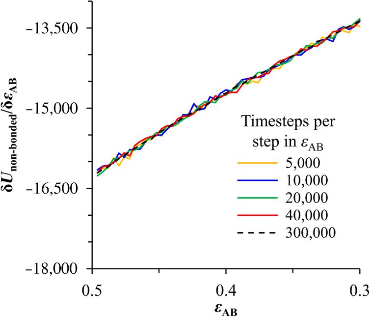

The third and final branch of each simulation gradually turns off the external potential. Equation (6) was then integrated where $u$ is $A$ as $A$ decreases from 2.6 to 0. This is described in Eq. (16).

Eq. (16)

$$\mathrm{\Delta }{F}_3=\underset{A_{\max }}{\overset{0}{\int }}\langle \tanh \left[\frac{\cos \left(\frac{2\pi x}{L}\right)}{2\pi w}\right]\rangle \mathrm{d}A.$$

This is the same as Eq. (13) except that the integration limits have been switched. The same analysis as was done in Fig. 4 is performed, the results of which are shown in Fig. 6. The integrand of Eq. (16) was calculated as a function of $A$ as $A$ was decreased for various numbers of time steps per step in $A$. Very low values of time steps per step in $A$ show significant deviations, but values of 20,000 and greater all produce the same integrand. This is consistent with the smaller morphological changes in branches two and three relative to branch one. The first branch was changed from a mixed state to an ordered state, while the second branch underwent almost no morphological change as $\chi$ was increased. This third branch, where the external potential is removed but $\chi$ is kept high, undergoes some minor morphological changes because there are some slight differences between the form of the external potential and the true defect. Therefore this integration was done in 50 steps and run for 40,000 ps for each step in $A$.

Fig. 6

Plot of the integrand of Eq. (16) as $A$ is decreased. Values of 20,000 timesteps per step in $A$ and higher yielded the same integrand.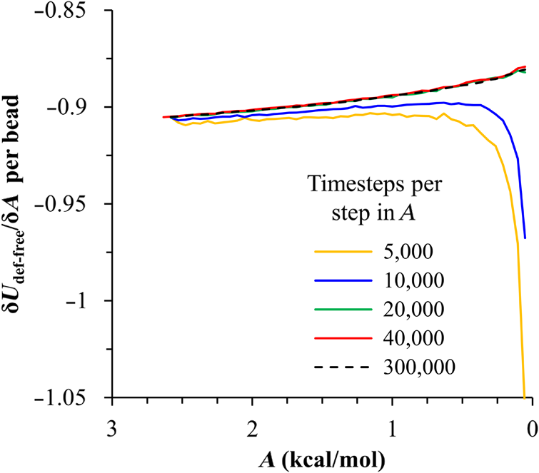

The free energies of each of these branches for both the mixed to defect and mixed to defect free simulations were calculated. $\mathrm{\Delta }{F}_1$, $\mathrm{\Delta }{F}_2$, and $\mathrm{\Delta }{F}_3$ are summed together to yield $\mathrm{\Delta }{F}_{\text{Defect}-\text{Mixed}}$ and $\mathrm{\Delta }{F}_{\text{DefectFree}-\text{Mixed}}$ as in Eq. (7).

3.

Results and Discussion

Various system sizes were simulated and the free energies were calculated to determine what system size was sufficient to accurately calculate the aforementioned free energy change. Box sizes in the $x$ direction, the dimension perpendicular to the aligned lamellae, were restricted to multiples of $L_0$ to preserve periodicity and commensurability with the natural pitch of the BCP lamellae. Whenever this dimension dropped to $3L_0$ or less, then the defect became severely distorted and free energy could not be calculated. Similar distortions occurred when the $y$ dimension decreased to very low values. Once the dimensions of the periodic box were greater than or equal to $5L_0$ in the $x$ dimension and $3L_0$ in the $y$ dimension, there did not seem to be a dependence of defect free energy on simulation area as shown in Fig. 7. This is very similar to box size constraints in the work of Nagpal et al.⁸ In these free energy measurements, there is some run to run variation, which is shown using 90% confidence interval error bars. The variation is likely caused by incomplete sampling in the given timeframe of calculation. If a simulation is temporarily trapped in a transition state, then that state will likely be oversampled causing a deviation in the calculation for that run. On average, either over very long simulations or over many simulations, the sampling would average out to be correct, but in finite runs and simulation time, sampling will not be perfect.

Fig. 7

Free energy of dislocation pair defect as a function of simulation size. Smaller simulation sizes resulted in deformed defects and made it impossible to calculate defect free energy. As long as the box size was at least $5L_0$ by $3L_0$ ($\text{area}=2160{\mathrm{nm}}^2$), the defect free energy did not vary significantly. The error bars shown are 90% confidence intervals over four or more simulations.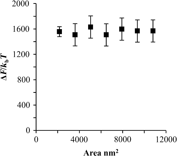

In order to determine the effect of $N$ and $\chi$ on the free energy of dislocation pairs, fully periodic simulations were run with box dimensions of $5L_0$ by $3L_0$ in the $x$ and $y$ dimensions and 15 nm in the film depth dimension. $L_0$ dimensions varied from $\sim 8.3$ to $\sim 23.1\mathrm{nm}$ (because of variations in $N$ and $\chi$). $N$ was varied from 64 monomers to 192 monomers at various $\chi$ values. The results are plotted as a function of $\chi N$ in Fig. 8. Defect free energy is usually investigated and reported as a function of $\chi N$, as it is done by Takahashi et al.⁷ However, as can be seen in this work (see Fig. 8), when both $N$ and $\chi$ are varied the defect free energies do not fall onto a single curve as a function of $\chi N$, but in fact show great disparities in defect free energy at a single $\chi N$. Linear extrapolations of the data in Fig. 8 yield intercepts (where the free energy of the defect and defect free state are equal) of $\chi N\sim 2$ to $\sim 11$ for each $N$ shown, but each set of $N$ only has 2 to 5 data points so the fits are subject to some error. In addition, values of $\chi N$ in this work generally stay above a $\chi N$ of 20, in part because defects very near the ODT had a tendency to very quickly heal themselves because of the very small or nonexistent barriers to defect healing.^22,29 However, the fact that the defect free energy approaches zero as the ODT is approached ($\chi N_{\mathrm{ODT}}\sim 10.5$) makes sense because as the drive to phase separate becomes small, the energetic penalties associated with the defect will become less and less important.

Fig. 8

The defect free energy as a function of $\chi N$. Overall, $\mathrm{\Delta }F$ increases with $\chi N$, but there is a significant change with $N$. Defect free energy approaches 0 as $\chi N$ approaches the ODT. Error bars represent 90% confidence interval.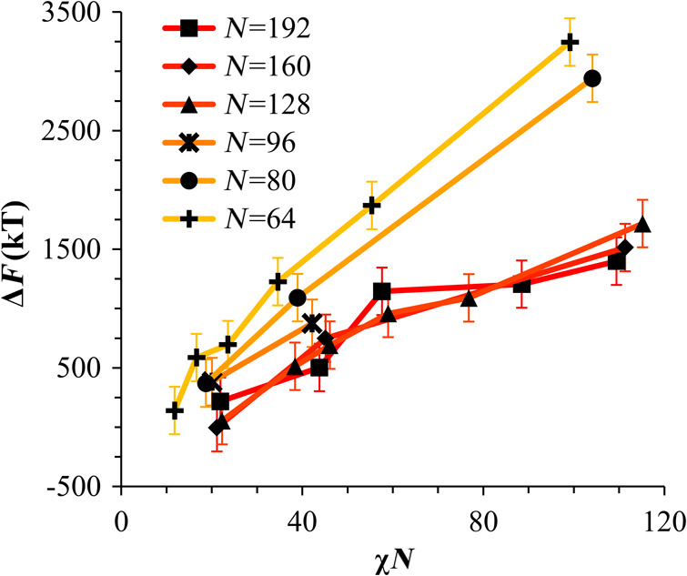

The size of the defect, when the thickness is fixed, as it is here, scales with $L_0^2$, and so one might expect that the defect free energy would scale with $\chi L_0^2$. The size of the defect scales with $L_0^2$ while the penalty for the defect might scale with $\chi$. However, as seen in Fig. 9(a), this scaling does not collapse the data to a single line. A second explanation for the variation might be that $\mathrm{\Delta }F$ scales with the increase in interfacial energy due to an increase in interfacial area due to the presence of the defect. The increase in interfacial energy can be represented by $\chi \mathrm{\Delta }I$, where $\mathrm{\Delta }I$ is the difference in the $A-B$ interfacial area between the defective and defect free state. The interfacial area between $A$ and $B$ lines increases linearly with $L_0$ as

Fig. 9

Defect free energy plotted versus (a) $\chi {\mathrm{L}}_0^2$ and (b) $\chi L_0$. Error bars are 90% confidence intervals.

When the same data are plotted as a function of solely $\chi$ as in Fig. 10, the data appear to collapse to a single curve. This is very surprising as it seems $L_0$, and therefore $N$ (which $L_0$ depends strongly) would be important as discussed above. There may be competing factors that appear to reduce the effect of $N$. For example, one might speculate that small chains may be stretched or compressed at the bends more than larger chains, which would increase the $\mathrm{\Delta }F$ for low $N$, but the effect of $L_0$ (which scales with $N^{\alpha }$ where $\alpha$ is between $2/3$ and $\sim 1$, depending on the value of $\chi N$³⁰) increases $\mathrm{\Delta }F$ for high $N$. These two factors would counteract each other, perhaps canceling each other out entirely. The idea that small chains are stretched or compressed more at the bends may be supported by the result that in polydisperse simulations, large chains concentrate near the bends and actually smooth the bends out some. This is shown later in this work in Fig. 14.

Fig. 10

(a) The defect free energy as a function of $\chi$. Defect free energy scales very well with $\chi$ with little dependence on $N$. Error bars show 90% confidence interval. (b) Fit line to the same data as in (a) with a 95% confidence interval on the fit shown as red lines.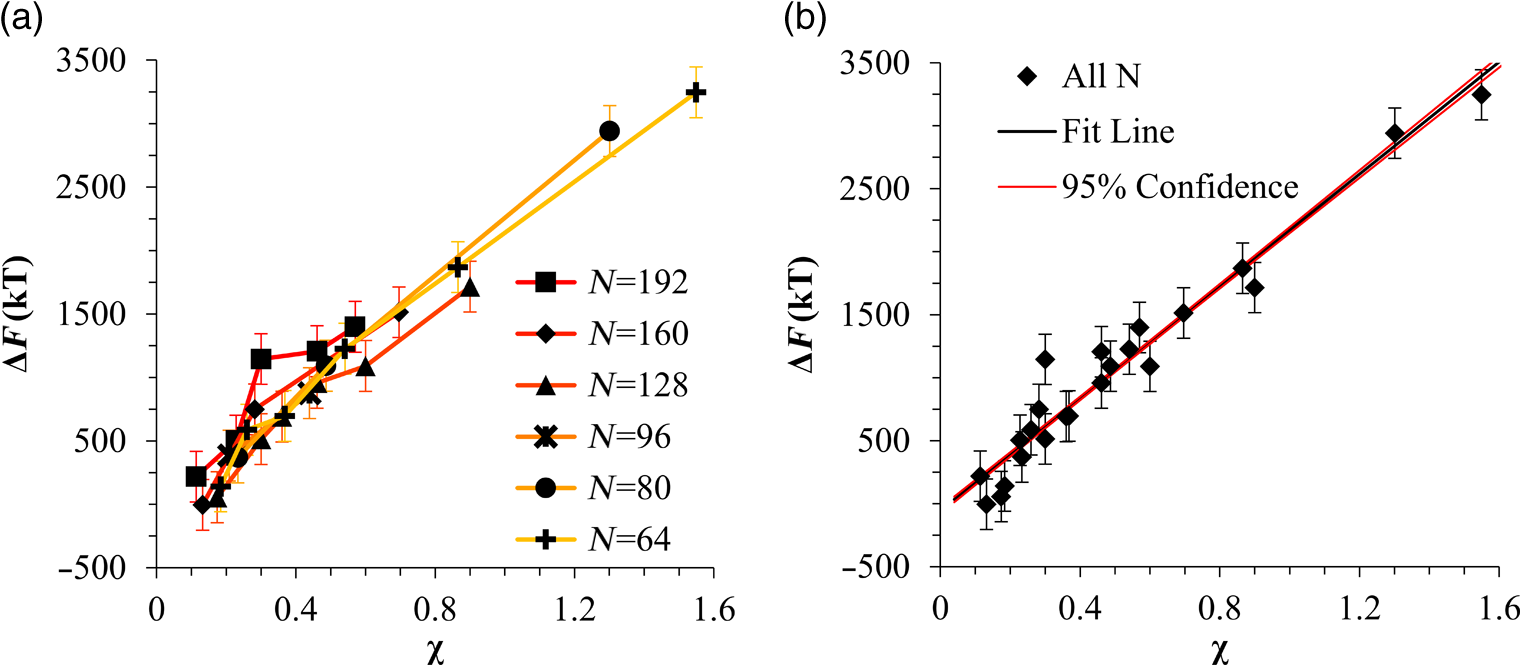

In order to produce smaller features, higher $\chi$ and lower $N$ materials are required to reduce the associated pitch. At a similar $\chi N$ value, but with a lower $N$ and a larger $\chi$, this data suggest the defect free energy will increase and therefore intrinsic defects will decrease. Previous work has shown that the energy barrier to defect removal is largely determined by $\chi N$ regardless of $N$^22,29 and decreasing $N$ will only speed up defect removal by increasing diffusive rates.²² That is, keeping $\chi N$ constant and reducing $N$ will increase defect annihilation rate as well as decrease the number of stable defects that will form. This means that future generations of DSA will likely suffer from fewer defect problems, assuming similar quality underlayers can be made for smaller features. Comparing the calculations here to defect densities for a known BCP may be useful. Processes using polystyrene-b-poly(methyl methacrylate) (PS-b-PMMA), the most commonly studied BCP for DSA, have obtained defect densities on the order of 1 defect ${\mathrm{cm}}^{-2}$.¹⁰ Extrapolating a fit to the data in Fig. 10 to a $\chi$ value of 0.04 (approximately the $\chi$ for PS-b-PMMA³¹) and using Eq. (1), a defect density of $\sim 0.001$ defects $\mathrm{per}{\mathrm{cm}}^2$ is obtained [using ${(10\mathrm{nm})}^2$ for the defect size]. However, this calculation does not account for imperfection in the guiding layers, the BCP, or the processing environment, which could potentially increase the defect density by several orders of magnitude.⁸ Accounting for these factors, and given the current state-of-the-art, experimentally achieved defect densities and the noise in this data, this calculated intrinsic defect density of PS-PMMA seems reasonable. Because the dependence of defect density on free energy is so strong, even a slight increase in $\chi$ and therefore in defect free energy results in defect densities that become vanishingly small.

The above results are obtained using fully periodic simulations so that the results are independent of guiding pattern. In order to explore the effect of guiding layers on defect free energy, thin film simulations were run. A thin film of BCP was placed over top of and in contact with a guiding layer composed of the same beads that compose the thin film of BCP. The underlayer was made to model a brush polymer covalently tethered to a hard substrate, as used previously.¹⁷ An underlayer with $2\times$ density multiplication, or a ratio of pinning stripe width to background region width of $1:3$ was used. These underlayers are composed of a pinning stripe that is preferential to one block and is 0.5 $L_0$ wide and a background region that is 1.5 $L_0$ wide. The LiNe process uses a similar pattern.³ Previous work by Nagpal et al.⁸ studied the effect of underlayer interaction strength with the film in the context of at $1:1$ pattern, that is alternating stripes each of width $L_0/2$. This type of pattern is not very useful in the context of semiconductor fabrication because the smallest feature size has already been achieved in the patterning of the underlayer (i.e., it does not multiple the density of the pattern). In industrially relevant processes at least one of the patterned stripes is wider than $L_0/2$ and the density of the pattern is multiplied via BCP-DSA. In processes, such as the LiNe process, the composition of the background region is varied to offer an underlayer that is more neutral overall to prevent horizontal lamellae from forming.¹⁹ Here, the effect of defect placement relative to the guiding pattern and the composition of the background region in the guiding pattern was measured, where the background region composition ($C_{\mathrm{b}}$) refers to the percent of the background region composed of the same bead that compose the pinning stripe. So, if the pinning stripe is composed of $A$ beads, then $C_{\mathrm{b}}=0\%$ means the background is all $B$ beads, while $C_{\mathrm{b}}$ 50% means the background region is equally composed of $A$ and $B$ beads. The dislocation pair defect can occur at three places on such an underlayer as shown in Fig. 11. In the “A placement,” the defect is centered on the pinning stripe. In the “B placement,” the pinning stripe is on the edge of the defect. The pinning line is shown under the left side of the defect in Fig. 11, but because the defect is symmetric this is identical to putting the stripe under the right side of the defect. In the “C placement,” the defect has the pinning stripes adjacent to both sides of the defect but not directly under the defect. Although the pinning stripes change from the $B$ block, to the $A$ block, and to the $B$ block in Fig. 11, the $A$ and $B$ blocks are energetically identical so it is merely an expedient to keep the defect unchanged and centered in the simulation volume. Defect free energies were calculated on these underlayers through various background compositions and the results are shown in Fig. 12 for $N=64$, $\chi N=35$, and a film thickness of $L_0$ (11 nm for this specific $N$ and $\chi N$).

Fig. 11

Images of the three possible defect locations on a $1:3$ guiding pattern.

Fig. 12

Defect free energy as a function of background composition and defect location relative to the underlayer for $N=64$, $\chi N=35$, and a film thickness of $L_0$ (11 nm). Error bars refer to 90% confidence interval about the mean.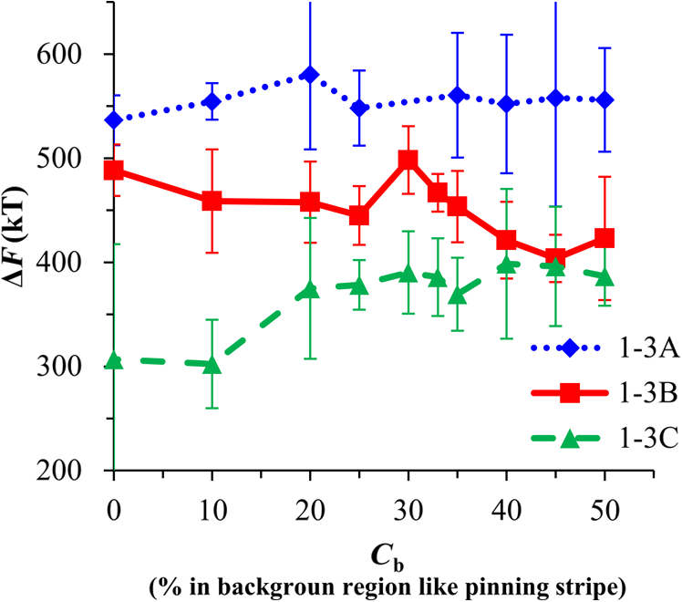

The defect location relative to the pinning stripes makes a significant difference in the measured free energy. When the pinning stripe is under the center of the defect (A placement), the free energy penalty is highest, followed by the pinning stripe being under one side of the defect (B placement) and finally pinning stripes that surround the defect (C placement). This effect can be explained by looking at how many lines the pinning stripe is influencing. For the A case, the pinning stripe interacts directly with one line (the line above it) and indirectly with the two adjacent lines. On the other hand, while in the B case the defect still directly interacts with one line, it only indirectly interacts with one adjacent line, which decreases the influence of the pinning stripe on the defect free energy. Finally, the C case does not directly influence any lines participating in the defect, but indirectly influences two adjacent lines, which further lowers the free energy of the defect.

The large differences in free energy as a function of defect placement relative to the underlayer ($\sim 100\mathrm{kT}$) on average means that the vast majority of defects will likely occur between pinning stripes (C placement) and not over top of them, although it appears that at higher background compositions defects with one edge over the pinning stripe (B placement) may appear in similar frequency. This result is significant because it is difficult to experimentally observe where defects form relative to the underlayer structure. At every background composition, the defects have very large penalties to form directly over the pinning stripe (A placement).

The effect of background region composition is not as clear. In the case of the A placement, background composition appears to have no significant effect on the free energy, while in the case of the B placement free energy appears to decrease with increasing $C_{\mathrm{b}}$, and in the C placement free energy appears to increase with increasing $C_{\mathrm{b}}$. However, the error bars are fairly large and make it difficult to claim such dependence with great certainty. From the simplest standpoint, where only the enthalpic interactions between the film and the underlayer are considered, the effect of $C_{\mathrm{b}}$ on the B placement makes sense. As $C_{\mathrm{b}}$ increases, the contrast (i.e., difference in composition) between the pinning stripe and the background region decreases and therefore decreases the guiding strength of the pattern. This would result in the defect free energy decreasing, as it is seen here. However, by this logic the defect free energy for the A placement should also decrease as $C_{\mathrm{b}}$ increases, but it does not. The C placement is different because no part of the defect directly touches the pinning stripe in this simplified view, so the pinning stripe would not impose a driving force to fix the defect. Any effect it does have will be through some less obvious means. This all suggests that something more complicated than the simple enthalpic interactions of the film with the underlayer is required to understand the effect that $C_{\mathrm{b}}$ has on $\mathrm{\Delta }F$. In previous works, it has been found that the shape of the interfaces is strongly affected by the underlayer composition,³² and changes at these interfaces have proven important in understanding the kinetics associated with defect removal.^31,32 In addition, these defects have a tendency to bend the lamellae slightly, even lamellae that are not immediately part of the defect (see Fig. 1: the first white lamellae not part of the defect are significantly bent) and the effect that this bend has on defect free energy is unclear. It may be that these interfacial changes are important to the defect free energy in these cases.

It should also be pointed out that these simulations have defect free energies less than half that of their periodic simulation counterparts (compare Fig. 12 with $N=64$ and $\chi N=35$ in Fig. 8). This is likely caused by the removal of interaction by the addition of the interfaces. Instead of having a dense polymer melt above and below the simulation volume, there is vacuum on one side and a thin brush on the other. This removes a large number of interactions that would affect the energy calculation. In addition, the density of the film near the free interface is depressed from its bulk density, further decreasing the overall number of interactions. Also, the fully periodic simulation is not analogous to a thin film on an unpatterned substrate because there are no interfaces, just interactions with the other side of the simulation volume. This means that the defect or defect free state essentially reinforces itself at the edge of the volume. The appearance of the film–underlayer interface and the film–vacuum interface plays an important role in defect free energy. This interface also proved critical in the study of defect healing kinetics.^10,31,33 We have also found that in some cases, defects that occur spontaneously have been accompanied by a local reduction in film thickness, but a thorough study has not yet been undertaken. This may also mean that film thickness plays an important role in defect free energy, but that was not directly studied here.

All simulations to this point were run with a molar mass dispersity ($\mathit{Ð}$) of 1, but in practice all BCPs have some molar mass dispersity. While it is expected that $\mathit{Ð}$ can increase the defectivity of a BCP film, this effect has not been explored in much detail. Previous work by Takahashi et al.⁷ studied the effect of $\mathit{Ð}$ (using binary blends of polymers) on the defect free energy in laterally confined BCPs. They found a decrease in $\mathrm{\Delta }F$ with $\mathit{Ð}$, and an interesting drop even at low $\mathit{Ð}$ as the ratio of masses of the blended polymers increased. However, using binary blends of polymers is very different from using a full distribution of lengths. Therefore, the effect that $\mathit{Ð}$ had on defect free energy was investigated using these simulations. Simulations using the B placement at $X_N=64$ ($X_N$ is the number average degree of polymerization) and $\chi N=35$ were built for various $\mathit{Ð}$ using a Wesslau distribution with chains randomly dispersed through the simulation. Each chain was forced to have a volume fraction of 50% A and B. The resulting defect free energies are shown in Fig. 13. There is a significant reduction in free energy with increasing $\mathit{Ð}$, to the extent that the defect free energy may approach or cross zero in value if $\mathit{Ð}$ were increased further. This implies that the defective state is as likely ($\mathrm{\Delta }F=0$) or more likely ($\mathrm{\Delta }F<0$) than the defect free state at very high $\mathit{Ð}$. At more commonly used $\mathit{Ð}$ values ($\mathit{Ð}=1.1$ or 1.2) the drop is still significant. At a $\mathit{Ð}$ of 1.2, the defect free energy has dropped almost 40% and would correspond to orders of magnitude increase in defect density. The work by Takahashi et al.⁷ saw a greater proportional drop at low $\mathit{Ð}$, but this drop in $\mathrm{\Delta }F$ did not approach 0 at high dispersity. This is likely caused by the fact that they used binary blends. In that work, it was found that larger differences in chains lengths lead to larger drops in $\mathrm{\Delta }F$. For our model with a full distribution, larger dispersities will include chains lengths with larger differences in length between them and so the effects of both larger differences in chain lengths and a broader distribution of such chains are felt.

Fig. 13

Defect free energy as a function of $\mathit{Ð}$ for $N=64$ and $\chi N=35$. The “B” defect location was used.

Figure 14 shows the locations of beads on long chains ($N>X_N$ where $X_N$ is the average chain length) and short chains ($N<X_N$) in a defect in a high dispersity case. There appears to be a higher concentration of long chains in the center of the defect than in the surrounding defect free areas. In addition, the defect seems more rounded and less angular than defects at lower dispersity. The distribution of various chain lengths appear to allow variations in line width (caused by variations in concentrations of chain lengths³⁴) that allow for smoother lines. This may stabilize the defect in a way similar to the way homopolymer additions stabilize bends in patterned block polymers.³⁵ This would imply that homopolymer additions would increase defect density at equilibrium.

Fig. 14

Distribution of chain lengths for $\mathit{Ð}=1.5$, $N=64$, and $\chi N=35$. Each point represents a single bead. The long chains tend to congregate near the defect.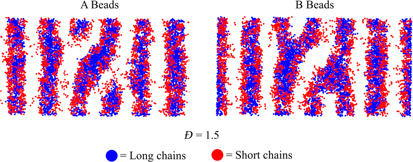

It should be pointed out that the external potential restricts almost all movement between lines so that chains are restricted to their original lines. They can move along an interface easily, but moving across an interface to another line would be a very rare event because of the high energetic penalty associated with moving a bead through the opposite typed domain. This has the effect of limiting variations in volume fraction and chain lengths from line to line through time. If at the actual lowest free energy state, the concentration of one length of chain is different near the defect as compared to far away from the defect, this distribution may not be properly sampled in the current simulations. This suggests the values calculated in Fig. 13 may be over estimates of the true defect free energy. A systematic examination of chain redistribution would discover if the lowest free energy state did redistribute some chains lengths closer to or farther from the defect. For example, creating a branch in the thermodynamic integration scheme that concentrated long or short chains near the defect, or increased the dispersity locally near the defect (but did not affect the overall dispersity) would help determine the distribution that would yield the lowest free energy state. However, such an examination was not performed here so the calculations show in Fig. 13 should be viewed as a maximum defect free energy.

4.

Conclusions

The defect free energy of a dislocation pair or jog defect is calculated via thermodynamic integration using a coarse-grained molecular dynamics model as a function of $\chi$ and $N$. It was found that $\chi N$ is not the best predictor of defect free energy and that a single $\chi N$ value can yield vastly different free energies when $\chi$ and $N$ are different (although their product is identical). This means that higher $\chi$ systems that are being produced to allow for smaller feature size DSA will likely have a lower equilibrium intrinsic defect density. Measurements of defect densities are reasonable for the oft-studied PS-PMMA. Defect free energies were measured as a function of defect placement relative to the underlayer and as a function of background composition. The effect of background composition was unclear but the defect free energy was highly dependent on defect location relative to the underlayer. Free energy differences of $\sim 100\mathrm{kT}$ were found between the three possible defect locations on a $1:3$ guiding pattern. The effect of $\mathit{Ð}$ on defect free energy was also studied. It was found that $\mathit{Ð}$ significantly reduced defect free energy. Long chains in a polydisperse sample tended to concentrate near and stabilize the defect.