Fast pixel-based optical proximity correction based on nonparametric kernel regression

Xu Ma; Bingliang Wu; Zhiyang Song; Shangliang Jiang; Yanqiu Li

doi:10.1117/1.JMM.13.4.043007

3 November 2014 Fast pixel-based optical proximity correction based on nonparametric kernel regression

Xu Ma, Bingliang Wu, Zhiyang Song, Shangliang Jiang, Yanqiu Li

Journal of Micro/Nanolithography, MEMS, and MOEMS, Vol. 13, Issue 4, 043007 (November 2014). https://doi.org/10.1117/1.JMM.13.4.043007

Abstract

Optical proximity correction (OPC) is a resolution enhancement technique extensively used in the semiconductor industry to improve the resolution and pattern fidelity of optical lithography. In pixel-based OPC (PBOPC), the layout is divided into small pixels, which are then iteratively modified until the simulated print image on the wafer matches the desired pattern. However, the increasing complexity and size of modern integrated circuits make PBOPC techniques quite computationally intensive. This paper focuses on developing a practical and efficient PBOPC algorithm based on a nonparametric kernel regression, a well-known technique in machine learning. Specifically, we estimate the OPC patterns based on the geometric characteristics of the original layout corresponding to the same region and a series of training examples. Experimental results on metal layers show that our proposed approach significantly improves the speed of a current professional PBOPC software by a factor of 2 to 3, and may further reduce the mask complexity.

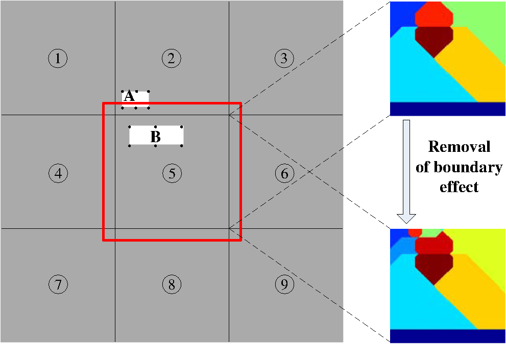
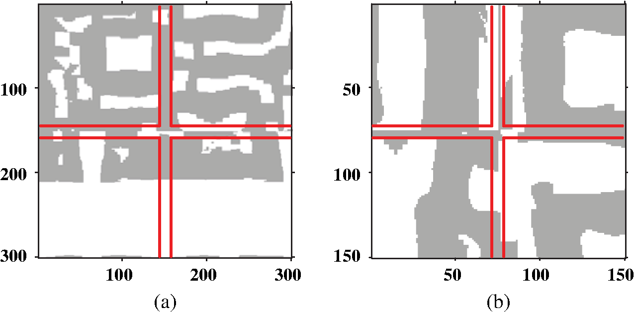
1. Introduction

The semiconductor industry has relied on resolution enhancement techniques (RET) to compensate and minimize mask distortions as they are projected onto semiconductor wafers.¹^–⁵ Resolution in optical lithography obeys the Rayleigh resolution limit $R = k_{1} (λ / NA)$ , where $λ$ is the wavelength, $NA$ is the numerical aperture, and $k_{1}$ is the process constant which can be minimized through RET methods.⁶^–¹⁵ Optical proximity correction (OPC) is one of the key RETs that modifies the mask pattern to precompensate for imaging distortions.

In general, OPC approaches are divided into two classes: rule-based and model-based approaches.² Rule-based approaches are mostly heuristic and are simple to implement, but can only compensate the warping in local features. On the other hand, model-based approaches use physical or mathematical models to represent the image formation process of the optical lithography system,¹⁶^,¹⁷ and iteratively seek the global minimization of the cost function to improve the image fidelity on the wafer. There are two types of model-based OPCs: edge-based OPC (EBOPC) and pixel-based OPC (PBOPC). EBOPC decomposes the mask into edges and corners and optimizes their locations, while pixel-based OPC decomposes the mask into small pixels and optimizes their transmission coefficients.¹⁸ Compared to EBOPC, PBOPC has more degrees of freedom during the optimization process, and may insert subresolution assistant features (SRAFs) around main mask features to further improve image fidelity.

In the past few decades, several PBOPC approaches have been proposed for advanced optical lithography to enhance the imaging performance at nominal settings¹⁹^–²⁷ or over a range of process variations.²⁸^–³¹ Although pixel-based approaches are effective for improving the imaging performance of lithography systems, these approaches are computationally intensive, especially for the current sophisticated large-scale masks. To alleviate this, a number of methods have been developed to accelerate the OPC design process. Frye et al. used neural networks to compensate for electron scattering effects in E-beam lithography systems resulting in a significant reduction in computation time as compared to iterative algorithms.³² Jedrasik proposed a neural network approach for one step OPC.³³ Recently, Huang et al. developed a method to train a neural network to map the fragment movements.³⁴ Gu and Zakhor generalized this idea and proposed a method based on linear regression to provide an initial estimate for the movement of edges and corners in EBOPC.¹⁸ Then, Gao et al. improved upon Gu and Zakhor by using principle component regression.³⁵ These initialization strategies can effectively reduce the number of iterations required for the EBOPC algorithms to converge and thereby reduce the overall runtime.¹⁸^,³⁵ These methods mentioned above opened a new line of research for efficient OPC solutions. However, it is desirable to use more advanced strategy to effectively improve the computational efficiency of PBOPC, which has many more degrees of freedom than EBOPC, for optical lithography systems.

In order to effectively speed up the current professional PBOPC software, this paper develops a fast PBOPC algorithm based on nonparametric kernel regression that is a well-known technique in machine learning. Our approach can be described as follows: First, training data are collected from the OPC pattern of a chip as computed by the professional PBOPC software Calibre pxOPC.³⁶ Subsequently, the test layout to be optimized is divided into three kinds of regions: convex corners, concave corners, and edges. Then, the nonparametric kernel regression is independently applied to these three kinds of regions. After that, the regression results are stitched up to compose the entire OPC pattern for the test layout. Finally, a postprocessing step is proposed to modify the regressed OPC pattern to further improve the image fidelity and to reduce the mask complexity. The proposed algorithm is tested using metal layers at 90- and 45-nm technology nodes. Simulations show that the proposed method significantly improves the speed of Calibre pxOPC software by a factor of 2 to 3, and may further reduce the mask complexity. It is noted that although the implementation of the proposed method is based on Calibre pxOPC software in this paper, the basic idea and fundamental framework can be extended to some other PBOPC approaches.

The remainder of this paper is organized as follows: the nonparametric kernel regression method used in our algorithm is discussed in Sec. 2. The training data collection process is described in Sec. 3. The fast PBOPC algorithm based on nonparametric kernel regression is developed in Sec. 4. Simulations are illustrated in Sec. 5, where the effects of the proposed algorithm on mask synthesis are shown. Conclusions are in Sec. 6.

2. Nonparametric Kernel Regression

2.1.

Regression Techniques

Suppose there are two sets of data $\vec{x}$ and $\vec{y}$ having the following relationship:

Eq. (1)

\vec{y} = f (\vec{x}) + \vec{ϵ},

where

f ()

is an arbitrary function and

\vec{ϵ}

is an error vector. Regression is a statistical technique which models the dependence of the output

\vec{y}

on the input features

\vec{x}

.³⁷ There are two classes of regression techniques: parametric and nonparametric. In parametric regression,

f ()

is assumed to be a global function with a known form but unknown parameters to be estimated. While parametric models such as linear regression remain the most popular techniques in data modeling, they are often too rigid to model general nonlinear patterns hidden in a high-dimensional data space.³⁸ On the other hand, nonparametric regression methods are suitable for nonlinear problems, where

f ()

is assumed to be a continuous function with an unknown form. The nonparametric regression methods directly estimate the regression function from the data rather than estimating the parameters.³⁹ PBOPC synthesis is a nonlinear problem in high-dimensional data space, and we apply nonparametric regression method to our proposed PBOPC algorithm.

2.2.

Nonparametric Kernel Regression

Nonparametric kernel regression is a well-known technique in machine learning. A variety of nonparametric regression approaches have been investigated in the literature.⁴⁰^,⁴¹ In this paper, we adopt the kernel-based nonparametric regression method in our algorithm. The Nadaraya–Watson kernel regression method was independently developed by Nadaraya and Watson, and takes the general form:⁴²^,⁴³

Eq. (2)

{\hat{\vec{y}}}_{t} = \hat{f} ({\vec{x}}_{t}) = \frac{\sum_{i = 1}^{N} {\vec{y}}_{i} K ({\vec{x}}_{t}, {\vec{x}}_{i})}{\sum_{i = 1}^{N} K ({\vec{x}}_{t}, {\vec{x}}_{i})},

where

{\vec{x}}_{i}

and

{\vec{y}}_{i}

are the input and output training data at hand,

{\vec{x}}_{t}

and

{\vec{y}}_{t}

are the input and output test data, and

K ({\vec{x}}_{t}, {\vec{x}}_{i})

is the kernel function. The training data imply the underlying relationship between the input and output, and are collected in advance to provide a priori knowledge for the test stage. The test data are the incoming data that are presumed to obey the input and output relationships inferred by the training data. The kernel method estimates the output test data

{\vec{y}}_{t}

based on the input test data

{\vec{x}}_{t}

and training data. A kernel function measures the similarity between the observations at

{\vec{x}}_{i}

and a given location

{\vec{x}}_{t}

, and weighs each

{\vec{y}}_{i}

to predict

{\vec{y}}_{t}

. Usually,

K ({\vec{x}}_{t}, {\vec{x}}_{i})

is a continuous, monotonically decreasing function with respect to the distance between

{\vec{x}}_{t}

and

{\vec{x}}_{i}

. There are many choices for

K ({\vec{x}}_{t}, {\vec{x}}_{i})

.⁴⁰ In this paper, we choose the Gaussian kernel

Eq. (3)

K ({\vec{x}}_{t}, {\vec{x}}_{i}) = \frac{1}{\sqrt{2 π}} \exp (- \frac{1}{2} {‖ \frac{{\vec{x}}_{t} - {\vec{x}}_{i}}{h} ‖}_{2}^{2}),

where

h

is the bandwidth to control the smoothing range. Particularly, in the PBOPC problem,

{\vec{x}}_{i}

is the sample vector of the training layout,

{\vec{y}}_{i}

is the optimized OPC pattern corresponding to

{\vec{x}}_{i}

,

{\vec{x}}_{t}

is the sample vector of the test layout, and

{\hat{\vec{y}}}_{t}

is the prediction of the OPC pattern due to the regression algorithm corresponding to

{\vec{x}}_{t}

. The training data collection method is described in the next section.

3. Training Data Collection

3.1.

Input Training Data Collection

We divide the layout data into two parts: training and testing. The training layout is used to build up the OPC training datasets to provide a priori knowledge for nonparametric kernel regression, while the test layout is the mask to be optimized. In this paper, we use two metal layers at 90- and 45-nm technology nodes in our simulations. In the future, we may investigate the proposed algorithm using test layouts with smaller critical dimensions (CD). Similar to Gu et al.,¹⁸ the features on the training layout are separated into three classes of fragments: convex corners, concave corners, and edges. In Fig. 1, the fragments shown in green, blue, and red are convex corners, concave corners, and edges, respectively. The input training data ${\vec{x}}_{i}$ consists of the samples around these fragments. The sampling centers of the convex and concave corners are set to be the convex and concave vertices, respectively, which are shown as points $O_{1}$ and $O_{2}$ in Fig. 1(a). The sampling center of the edge is selected as the midpoint of the edge boundary shown as $O_{3}$ . Generally, we denote the sampling center of each fragment as $O_{i}$ . In our simulations, we first scan the entire layout using the Calibre WORKbench window,³⁶ and save every snapped image of the layout with a resolution of 1 nm. Then, MATLAB^® is used to process the snaps and extract the coordinates of all convex and concave corners and edge centers.

Fig. 1

(a) Examples of the convex corner (left), concave corner (right), edge fragment (middle), and their sampling centers, where the sampling centers are shown by points $O_{1}$ , $O_{2}$ , and $O_{3}$ . (b) Examples of the observation points, where point A is the convex vertex, point B is the concave vertex, points C, D, and E are the observation points along the edge boundary. $L$ is the parameter to control the density of the observation points.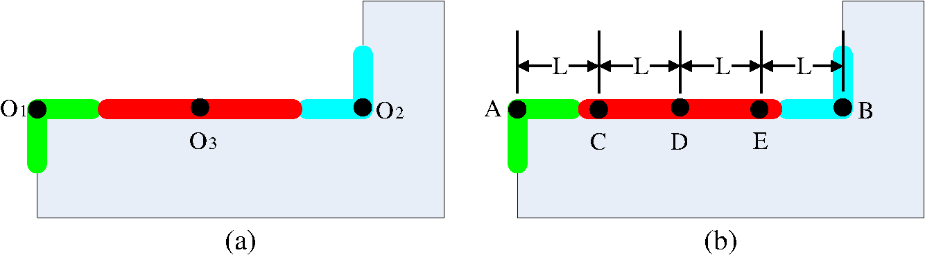

Around the sampling center $O_{i}$ , each fragment from the 90-nm metal layer is sampled at 5-nm per pixel in the surrounding $1.28 \times 1.28 {μ m}^{2}$ area, and each fragment from the 45-nm metal layer is sampled at 3-nm per pixel in the surrounding $0.768 \times 0.768 {μ m}^{2}$ area. As shown in Fig. 2(a), the sampling centers of the layout are illustrated by the red crosses. For each sampling center $O_{i}$ , we use an incremental concentric circular sampling method to sample its surrounding environment, where the sampling positions are located on a series of concentric circles around $O_{i}$ . Taking one of the convex corners as an example, we illustrate the corresponding sampling positions by black dots in Fig. 2(a). On each homocentric circle around $O_{i}$ , the layout is equally sampled in eight directions (up, down, left, right, up-left, up-right, down-left, and down-right). Since OPC is essentially an optical correction process, the intensity of light from a source will decrease along with the increment of the distance $| \vec{r} |$ from the source. For partially coherent illumination, the impact strength of a source decreases at a rate somewhere between $1 / | \vec{r} |$ and $1 / {| \vec{r} |}^{2}$ , depending on the level of partial coherence.¹ However, since we use relatively large partial coherence factors in our following simulations, for simplicity we approximately assume that the effects of a mask pattern on the wafer obey the inverse square law,³⁵ which means that the intensity of light from a source is proportional to $1 / {| \vec{r} |}^{2}$ .⁴⁴ In order to follow the quadratic pattern implied by the inverse square law, the radius $R_{j}$ of the $j$ ’th homocentric circle is increased as $R_{j} = pixel \times α^{j} nm$ , where pixel is the sampling pixel size that is equal to 5 and 3 nm for the 90- and 45-nm metal layers, respectively. $α$ is the parameter to control the distance between these homocentric circles. Therefore, the sampling density is reduced proportionally to the square of the distance from the sampling center. In our simulations, we choose $α = 2$ . In the sampling region, there are seven homocentric sampling circles, thus, 57 sampling points including the sampling center $O_{i}$ . Therefore, for each $O_{i}$ , we obtain an input training vector ${\vec{x}}_{i} \in B^{57}$ , where $B = {0,1}$ is the binary set.

Fig. 2

Relationships between the input training data and the output training data. (a) The input training data ${\vec{x}}_{i}$ obtained by the incremental concentric circular sampling method, and (b) the output training data ${\vec{y}}_{i}$ calculated by Calibre pxOPC. White and grey represent the openings and opaque areas, respectively. The locations of sampling centers are illustrated by the red crosses in both figures.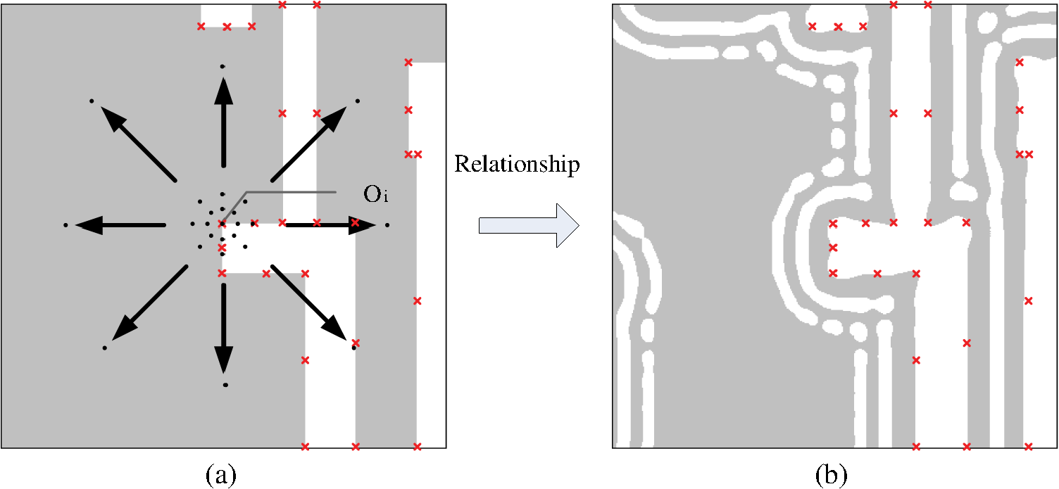

3.2.

Output Training Data Collection

The output training data ${\vec{y}}_{i}$ is the optimized OPC pattern corresponding to input training data ${\vec{x}}_{i}$ as described in Sec. 3.1. In this paper, the OPC pattern of training layout is obtained by using the professional software Calibre pxOPC. In practice, any other PBOPC approach would work. Our simulations are based on a vector optical model with wavelength $λ = 193 nm$ . For the 90-nm metal layer, we use a dry lithography system with $NA = 0.75$ , ambient refractive index of 1, and annular illumination with inner and outer partial coherence factors of $σ_{in} = 0.49$ and $σ_{out} = 0.79$ . For the 45-nm metal layer, we use an immersion lithography system with $NA = 1.35$ , ambient refractive index of 1.44, and annular illumination with inner and outer partial coherence factors of $σ_{in} = 0.584$ and $σ_{out} = 0.861$ . First, we run the Calibre pxOPC on the entire training layout. Then, for each sampling center $O_{i}$ on the layout, we capture its surrounding OPC pattern as shown in Fig. 2(b), where the red crosses indicate the locations of sampling centers corresponding to those in Fig. 2(a). For the 90-nm metal layer, the area of the surrounding OPC pattern is $3.0 \times 2.85 {μ m}^{2}$ and the pixel size is 5 nm; thus, the captured OPC pattern is translated into the output training vector ${\vec{y}}_{i} \in B^{342000}$ , where $B = {0,1}$ is the binary set. For the 45-nm metal layer, the area of the surrounding OPC pattern is $1.8 \times 1.8 {μ m}^{2}$ and the pixel size is 3 nm, therefore, the output training vector is ${\vec{y}}_{i} \in B^{360000}$ . Figure 2 shows the relationship between the input training data ${\vec{x}}_{i}$ and the output training data ${\vec{y}}_{i}$ . Based on this relationship, we construct three training datasets corresponding to convex, concave, and edge fragments, respectively. It is noted that the training data pairs of $({\vec{x}}_{i}, {\vec{y}}_{i})$ have a one-to-many relationship, where the same ${\vec{x}}_{i}$ may correspond to different ${\vec{y}}_{i}$ ’s. Basically, the one-to-many relationship results from two causes. The first reason is that we use 57 sampling points to represent the local geometries on the target pattern. Thus, the training datasets build a map from a sparse sampled space with a dimension of 57 to a large space with dimensions of the OPC examples. On the other hand, the second reason is that PBOPC synthesis is an ill-posed nonlinear problem, where numerous input patterns can lead to the same output pattern. This phenomenon is a physics-based reality that is independent of the proposed methodology. From this point of view, this one-to-many relationship guarantees the diversity of the training datasets, which is beneficial for searching the optimal OPC solution. The influence of the one-to-many relationship on the performance of the proposed algorithm will be investigated and discussed at length in our future work. According to Eq. (2), if several training data pairs with the same ${\vec{x}}_{i}$ are selected during the nonparametric regression process, the regressed OPC solution is the weighted average of the corresponding OPC examples denoted by ${\vec{y}}_{i}$ .

4. Fast Pixel-Based Optical Proximity Correction Algorithm

This section describes the test stage of the proposed fast PBOPC algorithm for a large-scale layout. As shown in Fig. 3, we first divide the entire layout into several smaller blocks. Each regressed OPC pattern is independently generated for each block using the method that will be described shortly in Secs. 4.1–4.3. Then, we stitch all of the OPC patterns together to obtain the entire OPC pattern for the large-scale layout. The stitch-up method will be described in Sec. 4.4. After that, we apply the postprocessing method in Sec. 4.5 to further improve the image fidelity and to reduce the mask complexity.

Fig. 3

Flowchart to solve for large-scale optical proximity correction (OPC) problem.

4.1.

Input Test Data Collection

The input test data are denoted by ${\vec{x}}_{t}$ , which represents the local geometric characteristics of the test layout. A portion of the metal layer is used for training, while another portion is used for testing. Given a test layout to be optimized, the goal of the proposed PBOPC algorithm is to synthesize its corresponding OPC pattern based on a nonparametric kernel regression method. The first step is to divide the entire layout into several smaller blocks as shown in Fig. 4. The left figure in Fig. 4 is the entire layout, which is divided into nine smaller blocks. For each block, we classify the features on the test layout into three types of fragments: convex corners, concave corners, and edges. Then, observation points are placed on the convex and concave vertices and along the edge boundaries. During the test phase, the nonparametric regression is independently performed around the convex, concave, and edge observation points. The regions surrounding all observation points on the test pattern are replaced by their regressed OPC solutions calculated by Eq. (2) to generate the output test data. An example of the observation points for the layout in Fig. 1(a) is illustrated in Fig. 1(b). In contrast to the input training data where there is only one sampling center for each edge, there could be multiple observation points along the edge in the input test data. The density of the observation points along the edges can be controlled by the parameter $L$ . If the distribution of observation points is too dense, the OPC design process becomes computationally intensive. However, if the distribution is too sparse, it is inadequate to capture the geometrical characteristics of the underlying layout, and degrades the OPC performance. In our simulations, for the 90-nm metal layer, we choose $L = 450 nm$ , while the edges shorter than 150 nm are ignored and no observation point is placed on them. For the 45-nm metal layer, we choose $L = 270 nm$ , while the edges shorter than 90 nm are ignored.

Fig. 4

Division of the large-scale layout and removal of the boundary effect.

The second step is to sample the test layout around these observation points using the incremental concentric circular sampling method as described in Sec. 3.1. An area around each observation point on the test layout is sampled to result in the input test data ${\vec{x}}_{t} \in B^{57}$ .

4.2.

Layout Decomposition

Given a block of the test layout, the nonparametric regression is independently performed around the convex, concave, and edge observation points. Thus, we need to decompose the test layout into a set of nonoverlapping regions spanned by different observation points. First, we set an initial region for each observation point. Figure 5(a) shows a part of the test layout with dimension of $1055 \times 675 nm$ and the observation points on it.⁴⁵ Figure 5(b) shows the initial region assigned to every observation point. For the convex and concave vertices, the initial regions are squares centered on the vertices with a side length of $w_{1} = CD$ , where CD is the minimum line width on the test layout. For the observation points on edges, the initial regions cover the edge boundaries with a thickness of $w_{1} = CD$ . Subsequently, all of the initial regions are extended to cover their surrounding areas. In particular, the initial regions are simultaneously extended in the four axis-parallel directions at the same speed. The extension ends when the prescribed maximum extension width $w_{2}$ , to be described shortly, is reached or one region starts to “hit” another one. If the extended regions are too large, unexpected artifacts appear around the region boundaries when generating the OPC pattern. On the other hand, if the extended regions are too small, some of the useful assist features around the main bodies in the layout are ignored. In our proposed algorithm, the maximum extension width $w_{2}$ is empirically chosen by users according to the OPC patterns in the training datasets, such that the extended areas include most of the assist features, while cutting off most of the undesired artifacts. In the following simulations, the maximum extension width is selected as $w_{2} = 400$ and 200 nm for the 90- and 45-nm metal layers, respectively. The decomposed pattern is referred to as the layout decomposition map. The decomposition map of the previous example is shown in Fig. 5(c). The goal of the layout decomposition is to cover all mask features with the decomposition map. However, the decomposition map cannot completely cover the centers of lines with a width larger than $2 (w_{1} + w_{2})$ , resulting in performance degradation. In order to fully cover the patterns of different layouts, the value of $w_{2}$ should be modified according to the maximum line width of the layout under consideration. In addition, the area of each piece in the decomposition map must be guaranteed to be smaller than the OPC examples in training datasets by adjusting the parameter $L$ in Fig. 1(b). Thus, the region supported by the OPC examples in training datasets described in Sec. 3.2 is large enough to cover the entire corresponding pieces in the decomposition map.

Fig. 5

An example of the layout decomposition map (adopted and modified from Ref. 45), (a) the observation points on a part of the test layout, (b) the initial regions assigned to the observation points, and (c) the layout decomposition map.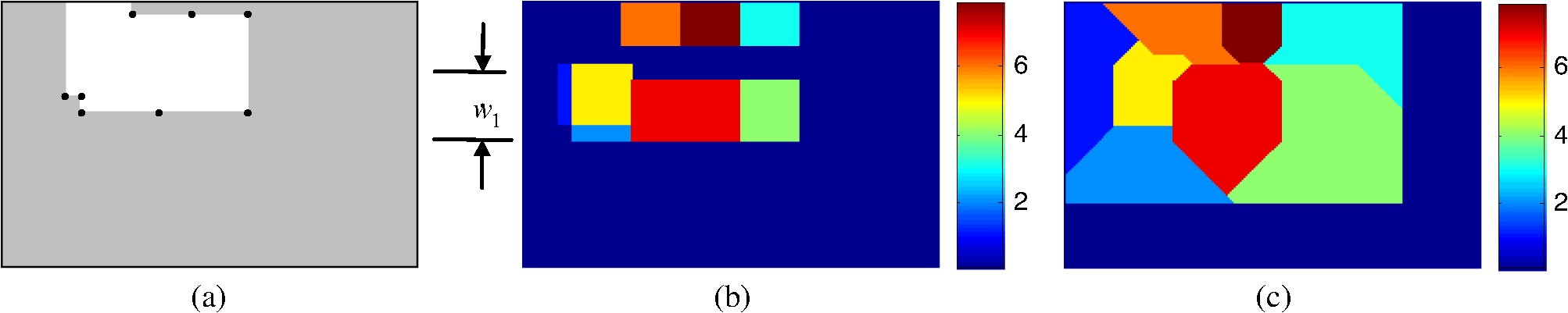

4.3.

Nonparametric Kernel Regression for Optical Proximity Correction Design

In Eq. (2), we substitute ${\vec{x}}_{i}$ and ${\vec{y}}_{i}$ with the input and output training vectors obtained in Sec. 3, and substitute ${\vec{x}}_{t}$ with the input test vector obtained in Sec. 4.1. Therefore, the output test vector ${\hat{\vec{y}}}_{t}$ is estimated by the kernel method, resulting in a continuously-valued PBOPC pattern. The value range of the pixels on the continuously-valued PBOPC pattern is $[0,1]$ . The continuously-valued ${\hat{\vec{y}}}_{t}$ from Eq. (2) is subsequently thresholded by 0.5, resulting in a binary OPC pattern. In our proposed algorithm, the nonparametric kernel regression is independently performed on convex corners, concave corners, and edges on the test layout. For each observation point, the regressed OPC pattern ${\hat{\vec{y}}}_{t}$ is truncated by the corresponding region on the layout decomposition map. In other words, each region on the map is filled in with the corresponding regressed OPC pattern computed via Eq. (2). Finally, all pieces of the regressed OPC patterns are stitched together without overlap to form the entire OPC pattern.

An illustrative example of the 90-nm metal layer is shown in Fig. 6. In the top row, Fig. 6(a) is a portion of the target pattern captured from the metal layer. Figure 6(b) is the corresponding PBOPC result calculated by the Calibre pxOPC software, where we run the “open” operation four times, the “decorate” operation six times, the “correction” operation six times, the “refine” operation six times, and the “manufacturing rule check (MRC)” operation 30 times. In the above flow, the “open,” “decorate,” “correction,” “refine,” and “MRC” are five jobs supported by Calibre pxOPC.³⁶ In particular, the “open” operation reshapes the layout features by growing the target shapes to ensure that the main feature is printable. The “decorate” operation adds initial SRAFs to improve the image quality. The “correction” operation corrects the image by suppressing extra-printings and improving the edge placement error (EPE) distribution on the main features. The “refine” operation performs fine-grained optimization for the best EPE root mean square and removes extra-printings. The “MRC” operation ensures that the final mask satisfies the predefined manufacturing constraints and the SRAFs do not print. Figure 6(c) is the regressed OPC pattern obtained by the proposed algorithm. In the bottom row, Figs. 6(d) to 6(f) are the print images on the wafer corresponding to the masks in Figs. 6(a) to 6(c), respectively. In this simulation, $N$ in Eq. (2) is set to be 5, and the bandwidth $h$ in Eq. (3) is to be 1. Another example of the 45-nm metal layer is shown in Fig. 7. In the Calibre pxOPC flow, we run the “open” operation once, the “decorate” operation six times, the “correction” operation eight times, the “refine” operation six times, and the “MRC” operation 30 times. The parameters of the proposed algorithm are the same as those in Fig. 6. In this paper, all of the print images on wafer are calculated by Calibre software. It is observed that the Calibre pxOPC software effectively improves the imaging performance and successfully achieves print images perfectly on target. However, as shown in Figs. 6(f) and 7(f), the print images of the regressed OPC patterns still include some residual bridges, gaps, and extra-printings as marked by the red boxes. That is because the regressed OPC pattern is composed by the weighted average of $N$ candidates chosen from the training datasets. Thus, some portions on the regressed OPC pattern are not optimal for the given optical and resist conditions. These portions usually introduce inferior image fidelity on the wafer. In addition, as shown in Figs. 6(c) and 7(c), the proposed method is apt to produce a lot of tiny and complex mask features that are difficult or even impossible to fabricate. In order to fix these problems, a postprocessing method is proposed in Sec. 4.5 to refine the raw regressed OPC pattern in order to improve the final image fidelity and to reduce the mask complexity.

Fig. 6

Performance comparison between Calibre pxOPC software and the proposed algorithm based on the 90-nm metal layer. From left to right, the top row shows: (a) a portion of the target pattern, (b) the PBOPC result calculated by Calibre pxOPC software, and (c) the regressed OPC pattern obtained by the proposed algorithm. In the bottom row, (d), (e) and (f) are the print images corresponding to the masks in (a), (b) and (c), respectively. White and black represent the openings and opaque areas, respectively.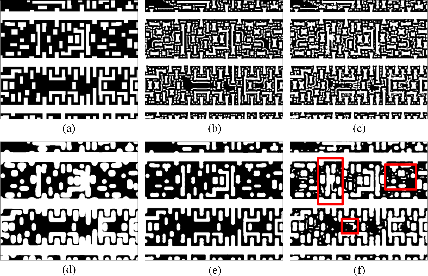

Fig. 7

Performance comparison between Calibre pxOPC software and the proposed algorithm based on the 45 nm metal layer. From left to right, the top row shows: (a) a portion of the target pattern, (b) the PBOPC result calculated by Calibre pxOPC software, and (c) the regressed OPC pattern obtained by the proposed algorithm. In the bottom row, (d), (e) and (f) are the print images corresponding to the masks in (a), (b) and (c), respectively. White and black represent the openings and opaque areas, respectively.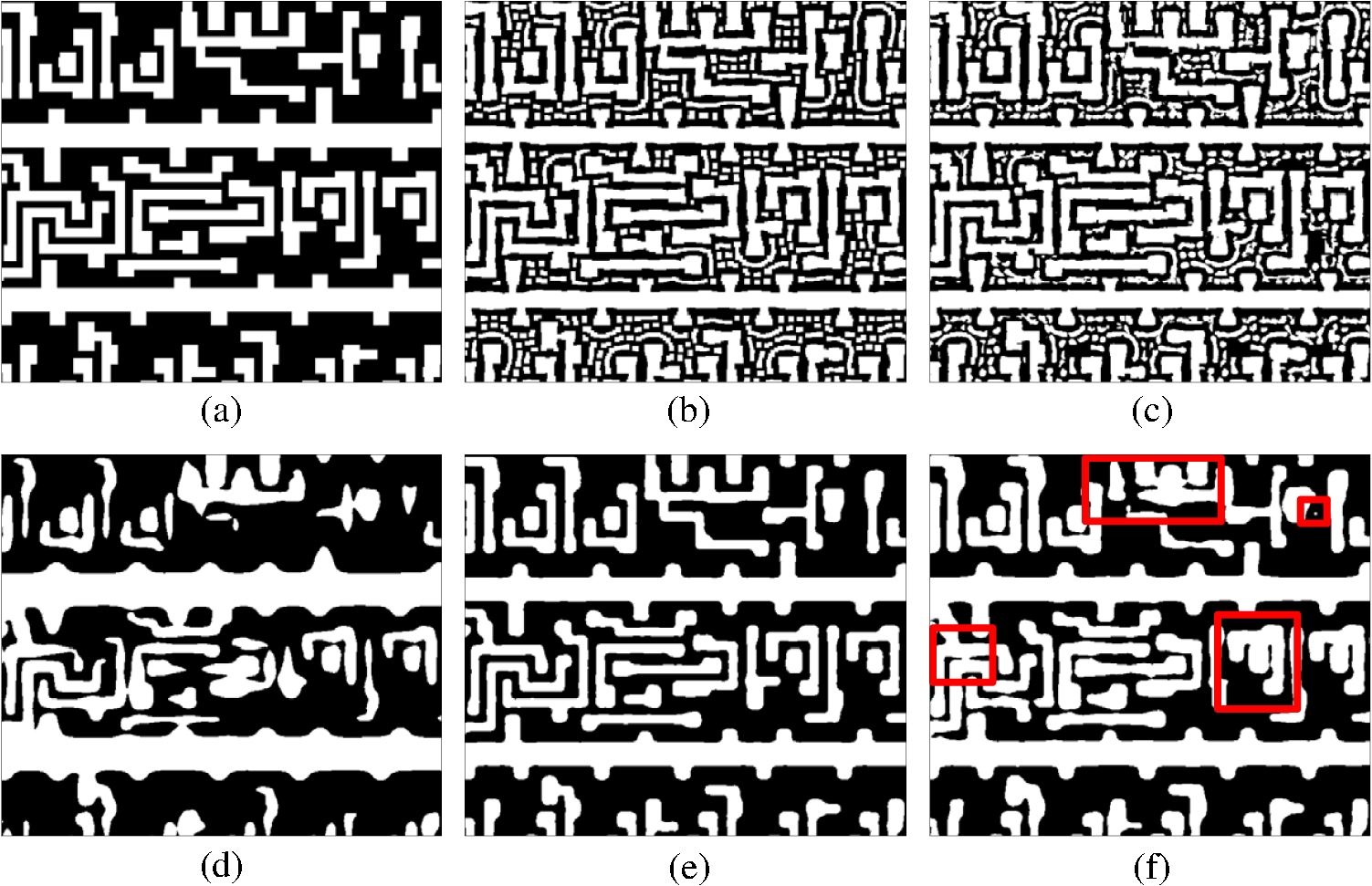

4.4.

Synthesis of Optical Proximity Correction Pattern for Large-Scale Layout

As shown in Fig. 3, each regressed OPC pattern is independently generated for each block using the method described in Secs. 4.1–4.3. Finally, we need to stitch all of the OPC patterns together to obtain the entire OPC pattern for the large-scale layout. As shown in Fig. 4, the left figure is the entire layout, which is divided into nine smaller blocks. Polygons $A$ and $B$ are located in blocks 2 and 5, respectively. Each polygon has six observation points as shown by the black dots. The three observation points in the lower part of polygon $A$ are very close to the boundary between blocks 2 and 5. In the layout decomposition map, the regions spanned by these observation points penetrate block 5. For the layout decomposition map of block 5, if we just take the six observation points on polygon $B$ , and ignore the influence of the three lower observation points on polygon $A$ , the boundary effect will be introduced, which is shown in the top right figure in Fig. 4. This naive layout decomposition map fails to include the influence of polygon $A$ . Therefore, when we stitch up the OPC patterns for all blocks, some assistant features around polygon $A$ may be truncated, degrading the imaging performance of the proposed algorithm.

The solution of the boundary effect is to include and consider the observation points within the external boundary surrounding each block. For example, when generating the layout decomposition map of block 5, we take all observation points inside the red square, which is extended from the original block in four directions. This method results in the revised layout decomposition map for block 5 as shown in the bottom right figure in Fig. 4. In the following simulations, we set the thickness of the external boundary of each block to be 650 nm for both 90- and 45-nm metal layers. Figures 8(a) and 8(b) show the connection of four regressed OPC blocks for the 90- and 45-nm metal layers, respectively. The stitch boundaries are located in the gaps between the red lines. Although the proposed method in this section can remove most of the boundary effects, some discontinuities of the OPC pattern still appear on the stitch boundaries. However, these mask discontinuities will be smoothed out by the following postprocessing method that will be described in next section.

Fig. 8

The connection of four regressed OPC blocks for the (a) 90-nm metal layer and (b) 45-nm metal layer.

4.5.

Postprocessing Method

As mentioned in Sec. 4.3, the OPC pattern directly synthesized by the nonparametric regression method is not optimal for the given optical and resist conditions, and usually introduces some residual bridges, gaps, and extra-printings in the print image. A bridge is the connection of separate patterns, and a gap is the disconnection of continuous patterns. Extra-printings are the unexpected imaging of the features that are disconnected from the target pattern. In this section, we propose a postprocessing method to further improve the image fidelity and to reduce the mask complexity. In general, the postprocessing method includes three steps as follows.

Step 1: Removal of extra-printings: Extra-printings are likely to appear at the positions where the SRAFs obtained by the regression method mismatch the optimal ones. This step removes the extra-printings by modifying the raw regressed OPC pattern according to the locations of these extra-printings. The print image of the raw regressed OPC pattern is first calculated by Calibre software, where all of the extra-printings on wafer are detected. We define the raw regressed OPC pattern as $A$ , and the extra-printings on the wafer as $B$ . Then the modified OPC pattern $C$ is calculated as
Eq. (4)
$C = A - (A & B),$
where & represents the intersection of the two arguments. By doing so, all SRAF areas overlapped with the extra-printings are eliminated.
Step 2: Mask patching and truncating: Since the regressed OPC pattern is calculated by a simple weighted average of training examples followed by a hard threshold operation, some irregular features, such as holes, notches, and protuberances arise in the regressed OPC pattern. These irregular features must be regularized, since they may dramatically increase the mask complexity and bring an inferior imaging performance onto the wafer. To achieve this goal, we first shrink the target pattern by 30 nm, and fill in all of the holes and notches inside the area supported by the shrunken target pattern. Subsequently, we dilate the target pattern outboard by 20 and 40 nm to form two contours, respectively. Then, we eliminate all the mask protuberances attached to mainbody features (rather than SRAFs) between the two contours mentioned above.
Step 3: Corner correction: The modified regressed OPC pattern from the previous two steps is input to the Calibre pxOPC software, and a few optimization iterations are carried out to refine the mask corners in order to further improve the image fidelity. In particular, we run the “refine” operation four times to modify the mask corners of the 90-nm metal layer, while we run the “correction” operation two times and the “refine” operation six times for the 45-nm metal layer. Then, the MRC function of Calibre is applied to impose the manufacturing constaints on the modified OPC pattern and to finalize the postprocessing. We assign the MRC parameters as follows: $mrc_iterations = 30$ , $mrc_\min_edge = 0.04 μ m$ , $mrc_\min_internal = 0.02 μ m$ , and $mrc_\min_external = 0.04 μ m$ . The “correction” and “refine” operations have been explained in Sec. 4.3. Compared to the Calibre pxOPC flows described in Sec. 4.3, the nonparametric regression method saves four “open” operations, six “decorate” operations, six “correction” operations, and two “refine” operations for the 90-nm metal layer, while it saves one “open” operation, six “decorate” operations, and six “correction” operations for the 45-nm metal layer.

The top and bottom rows of Fig. 9 illustrate the results of the postprocessing method for the 90- and 45-nm metal layers, respectively. For the 90-nm metal layer, the raw regressed OPC pattern before postprocessing is shown in Fig. 6(c). Figures 9(a) and 9(b) are the modified OPC patterns after applying Steps 2 and 3 mentioned above, and Fig. 9(c) is the final print image after applying the postprocessing method. For the 45-nm metal layer, the raw regressed OPC pattern is shown in Fig. 7(c). Figures 9(d) and 9(e) are the modified OPC patterns after applying Steps 2 and 3, and Fig. 9(f) is the final print image after applying the postprocessing method. It is observed from Figs. 6, 7, and 9 that the image fidelities of the regressed OPC patterns after postprocessing are similar to those obtained by the Calibre pxOPC software. In addition, the postprocessing method can effectively reduce the complexity of the optimized mask patterns.

Fig. 9

The results of the postprocessing method for the 90- and 45-nm metal layers. The top row shows the resulting OPC patterns for 90-nm metal layer after applying (a) Step 2 and (b) Step 3, and (c) the final print image after applying the postprocessing method. The bottom row shows the resulting OPC patterns for 45-nm metal layer after applying (d) Step 2 and (e) Step 3, and (f) the final print image after applying the postprocessing method. White and black represent the openings and opaque areas, respectively.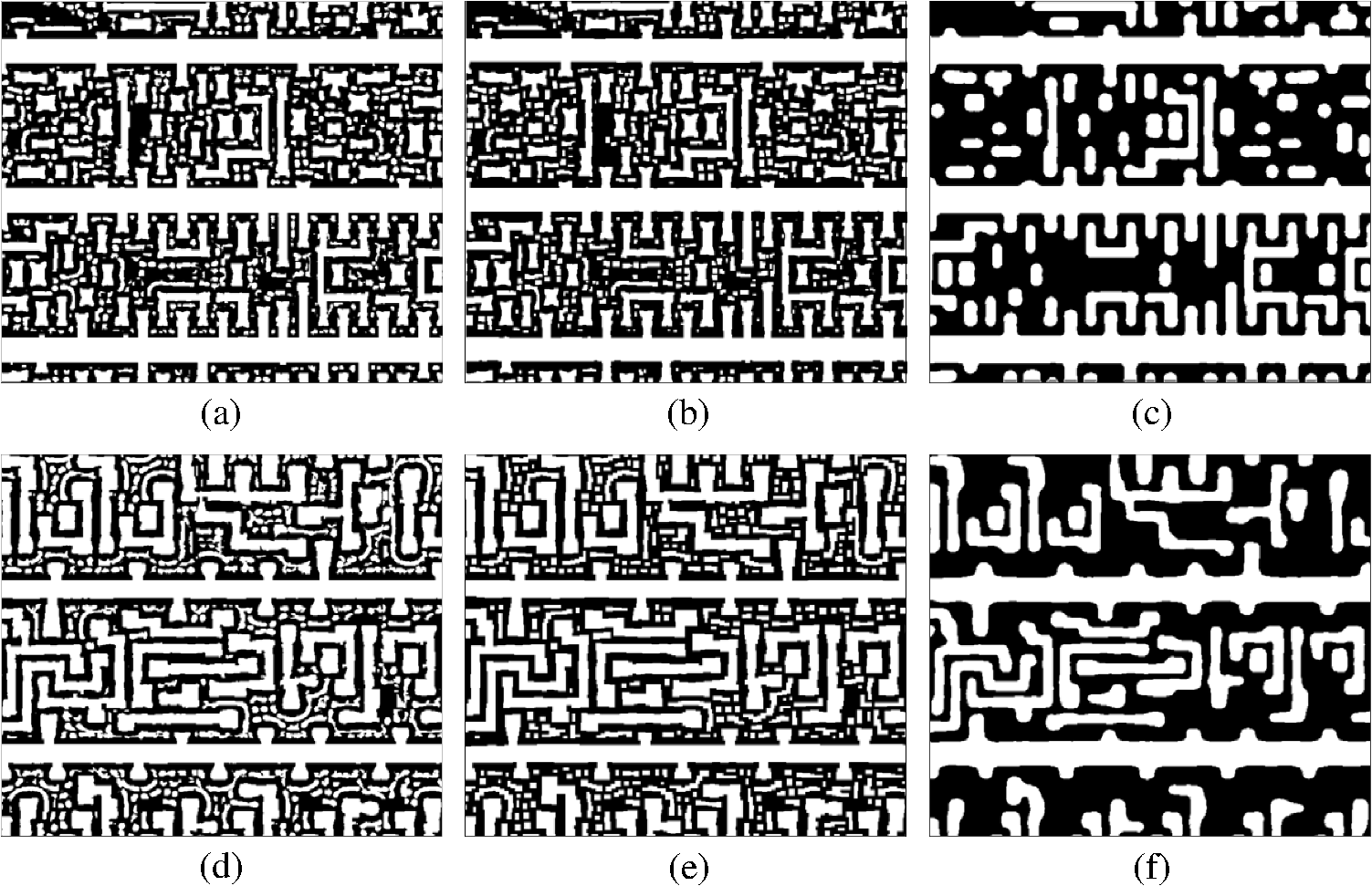

5. Simulations

In this section, we present the simulations of the proposed OPC method based on nonparametric kernel regression using the 90- and 45-nm metal layers. Then we compare the performance of Calibre pxOPC software and the proposed method with respect to the image fidelity, computational efficiency, and mask complexity. In the following simulations, the parameters of the optical models are the same as those described in Sec. 3.2. For the 90-nm metal layer, a $42 \times 36 {μ m}^{2}$ portion in the right area of the entire layout serves as the training pattern to build the training dataset. The training dataset includes 4000 convex vertices, 2000 concave vertices, and 10,000 edge fragments. A $48 \times 45.6 {μ m}^{2}$ region captured from the central area of the entire layout is used as the test pattern to be optimized. We divide the test pattern into $16 \times 16$ smaller blocks, each of which has dimensions of $3 \times 2.85 {μ m}^{2}$ . The proposed algorithm is performed on each of the smaller blocks. The entire OPC pattern is composed by aligning and stitching up all OPC patterns for each block without overlapping. For the 45-nm metal layer, a $42 \times 42 {μ m}^{2}$ portion in the right area of the entire layout is used as the training pattern. The training dataset includes 6000 convex vertices, 4000 concave vertices, and 10,000 edge fragments. A $14.4 \times 14.4 {μ m}^{2}$ region captured from the central area of the entire layout is used as the test pattern. We divide the test pattern into $8 \times 8$ smaller blocks, each of which has dimensions of $1.8 \times 1.8 {μ m}^{2}$ . In order to further accelerate the proposed algorithm, we translate all output training data into binary files, and read all training data into memory before the regression process. Thus, our program can load training data directly from memory rather than from the hard drive. As an example, the simulation results corresponding to a small portion on the 90- and 45-nm metal layers have been provided in Figs. 6, 7, and 9. In these simulations, $N$ in Eq. (2) is set to be 5, and the bandwidth $h$ in Eq. (3) is 1. Other parameters of the proposed algorithm have been described in Sec. 4. Based on these illustrative results, we conclude that the OPC solutions and print images resulting from the proposed algorithm and Calibre pxOPC are visually similar.

In the following, we quantitatively compare the performance between the proposed algorithm and Calibre pxOPC software with respect to image fidelity, computational efficiency, and mask complexity. We first use the metric of EPE and the pattern error to compare the image fidelity performance between these two methods. The pattern error is defined as the area of the difference region between the print image and the target pattern. We use Calibre to detect and collect all sites on the print images with an absolute EPE value ( $| EPE |$ ) larger than 3 nm. Then, we normalize the site number to 2000 and plot the histograms in Fig. 10 to show the distributions of $| EPE |$ values. Figures 10(a) and 10(b) are the histograms for the 90- and 45-nm metal layers, respectively. Table 1 summarizes the distributions of $| EPE |$ values for these 2000 detected sites with different methods. The initial mask patterns without optimization lead to many large $| EPE |$ values falling in the range of [20, 35 nm), while the Calibre pxOPC and the proposed algorithm can effectively suppress the $| EPE |$ values by concentrating most of them into the range of [0, 20 nm). The third row of Table 2 provides the average $| EPE |$ values, which is defined as the sum of all $| EPE |$ values divided by the detected site count. The fourth row of Table 2 provides the pattern errors. For the 90-nm metal layer, compared to the initial mask pattern, Calibre pxOPC and the proposed algorithm may reduce the average $| EPE |$ by 84% and 81%, while reducing the pattern error by 93% and 92%, respectively. The average $| EPE |$ and pattern error of the proposed algorithm are 16% and 21% higher than Calibre pxOPC. For the 45-nm metal layer, compared to the initial mask pattern, Calibre pxOPC and the proposed algorithm may reduce the average $| EPE |$ by 62% and 58%, while reducing the pattern error by 83% and 81%, respectively. The average $| EPE |$ and pattern error of the proposed algorithm are 12% and 10% higher than Calibre pxOPC. According to the above analysis, both of the Calibre pxOPC and proposed algorithm can effectively reduce the $| EPE |$ in contrast to the initial mask pattern. In addition, the image fidelity of Calibre pxOPC is better than that of the proposed algorithm. The computational efficiency of different methods is compared in the following. All of the computations are carried out on an Intel(R) Xeon(R) x5650 CPU, 2.67 GHz, 32.00 GB of RAM. The nonparametric regression process of the proposed algorithm is implemented in C language, and the postprocessing is implemented by the Calibre software. The test layouts are saved as OASIS files. In order to fairly compare the runtimes, we removed the hierarchies in the OASIS files, and ran both of the Calibre software and C codes using one CPU core. The runtimes of Calibre pxOPC and the proposed algorithm are summarized in the fifth row of Table 2. For the simulations of 90-nm metal layer, the Calibre pxOPC and the proposed algorithm took 1910 and 991 s, respectively. In particular, the nonparametric regression process based on the C language took 219 s. In the postprocessing method, Steps 1 and 2 together took 20 s, and Step 3 took 752 s. For the simulations of 45-nm metal layer, the Calibre pxOPC and the proposed algorithm took 881 and 341 s, respectively. The nonparametric regression process based on C language took 99 s. In the postprocessing method, Steps 1 and 2 together took 7 s, and Step 3 took 235 s. Compared to the Calibre pxOPC, the proposed algorithm reduced the runtime by 48% and 61% for the 90- and 45-nm metal layers, respectively. It is also noted that the times to build up the OPC training datasets are 10.0 and 11.6 h for the 90- and 45-nm metal layers, respectively. However, whenever the training datasets are built up, they can be repeatedly applied for different layers with similar geometric characteristics.

Fig. 10

Histograms of the $| EPE |$ values corresponding to the target pattern and OPC patterns obtained by the Calibre pxOPC and the proposed algorithm for the (a) 90-nm metal layer and (b) 45-nm metal layer, respectively.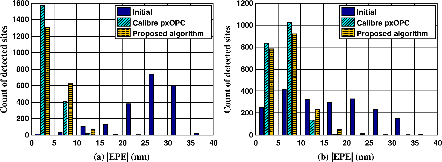

Table 1

The distributions of the |EPE| values for different methods. |EPE| is the absolute EPE value, and #|EPE| means the count of detected sites.

# $\| EPE \|$ within	Initial		Calibre pxOPC		Proposed
# $\| EPE \|$ within	90 nm	45 nm	90 nm	45 nm	90 nm	45 nm
(0, 5 nm)	8	249	1574	837	1300	784
(5, 10 nm)	29	415	411	1024	629	919
(10, 15 nm)	101	321	15	135	64	234
(15, 20 nm)	130	299	0	4	6	50
(20, 25 nm)	378	328	0	0	1	10
(25, 30 nm)	738	230	0	0	0	2
(30, 35 nm)	602	154	0	0	0	1
$\geq 35 nm$	14	4	0	0	0	0

Table 2

Performance comparison between Calibre pxOPC and the proposed algorithm.

Criterion	Initial		Calibre pxOPC		Proposed
Criterion	90 nm	45 nm	90 nm	45 nm	90 nm	45 nm
Average $\| EPE \|$ (nm)	26.5	15.9	4.3	6.0	5.0	6.7
Pattern error ( $μ m^{2}$ )	388.7	28.0	26.2	4.9	31.7	5.4
Runtime (s)	—	—	1910	881	991	341
Trapezoid count	3822	1361	89830	15769	87511	10974

In the following, we adopt the trapezoid count in the fractured masks as the metric to evaluate the mask complexity of different methods, where fewer trapezoids mean lower mask complexity.³⁶^,⁴⁶ We used the mask data preparation function of the Calibre software to fracture the initial mask pattern and the optimized OPC patterns obtained by the Calibre pxOPC and proposed algorithm. The parameter “Small Value” in Calibre was set as 20 nm to define the threshold of external slivers. The resulting trapezoid counts are presented in the sixth row of Table 2. In contrast to Calibre pxOPC, the proposed algorithm may reduce the trapezoid counts by 3% and 30% for the 90- and 45-nm metal layers, respectively. This means the proposed algorithm may further reduce the mask complexity compared to Calibre pxOPC. From the simulation results and analysis above, we conclude that the proposed algorithm can effectively speed up the current professional Calibre pxOPC software and reduce the resulting mask complexity. However, the gain of computational efficiency and mask simplicity is at the cost of acceptable image fidelity degradation. In the future work, we will try to adjust the parameters in our proposed method and the Calibre pxOPC flow to further reduce the image accuracy gap between these two methods, and try to compare the performance of the two methods based on a fixed image error. In the future, we will also investigate the application of the proposed algorithm in more advanced technology nodes, and study the key factors influencing the capacity and scalability of the algorithm, such as the density, diversity, and dimension of the layout, as well as the polygon counts included in the mask.

6. Conclusion

This paper developed a fast OPC algorithm based on a nonparametric kernel regression method. First, the input training data were sampled from the training layout, and the output training data were collected from Calibre pxOPC. The OPC training datasets were established for convex corners, concave corners, and edges, respectively. Subsequently, the test layout was divided into different regions spanned by a set of observation points. Then, the nonparametric kernel regression was independently performed for each of the regions. The final OPC for the entire test layout was generated by stitching up all pieces of regressed OPC patterns. In order to further improve the image fidelity and to reduce the mask complexity, a postprocessing step was applied to modify the raw regressed OPC pattern. In this paper, both the 90- and 45-nm metal layers were used to test and investigate the proposed algorithm. Simulations illustrated that compared to Calibre pxOPC software, the proposed method may achieve approximately a twofold to threefold speed up and a lower mask complexity at the cost of acceptable image fidelity degradation. However, our current work focuses on improving the image fidelity at nominal conditions without considering the process variations of lithography systems. In future work, we would generalize the proposed algorithm to extend the process window under defocus and dose variation.

Acknowledgments

We appreciate the support from Professor Avideh Zakhor and Mr. Shangliang Jiang at UC Berkeley. We thank the financial support by Key Program of National Natural Science Foundation of China under No. 60938003, the National Science and Technology Major Project, Program of Education Ministry for Changjiang Scholars in University, the National Natural Science Foundation of China (Grant No. 61204113), the Program for New Century Excellent Talents in University (NCET, Grant No. NCET-10-0042), the Special Plan of Major Project Cultivation of Beijing Institute of Technology, the Basic Research Foundation of Beijing Institute of Technology (Grant No. 20120442001), and the Technology Foundation for Selected Overseas Chinese Scholar. We also thank Mentor Graphics Corporation for providing academic use of Calibre.

References

1.

A. K. Wong, Resolution Enhancement Techniques in Optical Lithography, SPIE Press, Bellingham, Washington (2001). Google Scholar

2.

Computational Lithography, Wiley Series in Pure and Applied Optics, 1st ed.John Wiley and Sons, New York (2010). Google Scholar

3.

Y. Liet al., “Vectorial resolution enhancement: better fidelity for immersion lithography,” SPIE Newsroom, (2014). http://dx.doi.org/10.1117/2.1201409.005461 Google Scholar

4.

X. Guoet al., “Co-optimization of the mask, process, and lithography-tool parameters to extend the process window,” J. Micro/Nanolith. MEMS MOEMS, 13 (1), 013015 (2014). http://dx.doi.org/10.1117/1.JMM.13.1.013015 JMMMGF 1932-5134 Google Scholar

5.

Y. Liet al., “The cross talk of multi-errors impact on lithography performance and the method of its control (invited paper),” Proc. SPIE, 8418 841802 (2012). http://dx.doi.org/10.1117/12.978295 PSISDG 0277-786X Google Scholar

6.

S. A. Campbell, The Science and Engineering of Microelectronic Fabrication, 2nd ed.Publishing House of Electronics Industry, Beijing, China (2003). Google Scholar

7.

F. Schellenberg, “Resolution enhancement technology: the past, the present, and extensions for the future,” Proc. SPIE, 5377 1 –20 (2004). http://dx.doi.org/10.1117/12.548923 PSISDG 0277-786X Google Scholar

8.

F. Schellenberg, Resolution Enhancement Techniques in Optical Lithography, SPIE Press, Bellingham, Washington (2004). Google Scholar

9.

L. Liebmannet al., “TCAD development for lithography resolution enhancement,” IBM J. Res. Develop., 45 651 –665 (2001). http://dx.doi.org/10.1147/rd.455.0651 IBMJAE 0018-8646 Google Scholar

10.

J. LiS. LiuE. Lam, “Efficient source and mask optimization with augumented lagrangian methods in optical lithography,” Opt. Express, 21 8076 –8090 (2013). http://dx.doi.org/10.1364/OE.21.008076 OPEXFF 1094-4087 Google Scholar

11.

S. LiX. WangY. Bu, “Robust pixel-based source and mask optimization for inverse lithography,” Opt. Laser Technol., 45 285 –293 (2013). http://dx.doi.org/10.1016/j.optlastec.2012.06.033 OLTCAS 0030-3992 Google Scholar

12.

J. LiY. ShenE. Lam, “Hotspot-aware fast source and mask optimization,” Opt. Express, 20 21792 –21804 (2012). http://dx.doi.org/10.1364/OE.20.021792 OPEXFF 1094-4087 Google Scholar

13.

Y. Penget al., “Gradient-based source and mask optimization in optical lithography,” IEEE Trans. Image Proc., 20 2856 –2864 (2011). http://dx.doi.org/10.1109/TIP.2011.2131668 IIPRE4 1057-7149 Google Scholar

14.

N. JiaE. Y. Lam, “Pixelated source mask optimization for process robustness in optical lithography,” Opt. Express, 19 19384 –19398 (2011). http://dx.doi.org/10.1364/OE.19.019384 OPEXFF 1094-4087 Google Scholar

15.

Z. Songet al., “Inverse lithography source optimization via compressive sensing,” Opt. Express, 22 14180 –14198 (2014). http://dx.doi.org/10.1364/OE.22.014180 OPEXFF 1094-4087 Google Scholar

16.

L. DongY. LiX. Guo, “Influence of the axial component of mask diffraction spectrum on lithography imaging,” Acta Opt. Sin., 33 1111002 (2013). http://dx.doi.org/10.3788/AOS GUXUDC 0253-2239 Google Scholar

17.

L. YangY. LiK. Liu, “Simulation of the polarization effects induced by the bilayer absorber alternating phase-shift mask in conical diffraction,” Opt. Eng., 52 (9), 091702 (2013). http://dx.doi.org/10.1117/1.OE.52.9.091702 OPEGAR 0091-3286 Google Scholar

18.

A. GuA. Zakhor, “Optical proximity correction with linear regression,” IEEE Trans. Semicond. Manuf., 21 263 –271 (2008). http://dx.doi.org/10.1109/TSM.2008.2000283 ITSMED 0894-6507 Google Scholar

19.

S. SherifB. SalehR. Leone, “Binary image synthesis using mixed integer programming,” IEEE Trans. Image Proc., 4 1252 –1257 (1995). http://dx.doi.org/10.1109/83.413169 IIPRE4 1057-7149 Google Scholar

20.

Y. LiuA. Zakhor, “Binary and phase shifting mask design for optical lithography,” IEEE Trans. Semicond. Manuf., 5 138 –152 (1992). http://dx.doi.org/10.1109/66.136275 ITSMED 0894-6507 Google Scholar

21.

Y. Granik, “Solving inverse problems of optical microlithography,” Proc. SPIE, 5754 506 –526 (2004). http://dx.doi.org/10.1117/12.600141 PSISDG 0277-786X Google Scholar

22.

Y. Granik, “Fast pixel-based mask optimization for inverse lithography,” J. Micro/Nanolith. MEMS MOEMS, 5 (4), 043002 (2006). http://dx.doi.org/10.1117/1.2399537 JMMMGF 1932-5134 Google Scholar

23.

A. PoonawalaP. Milanfar, “Mask design for optical microlithography: an inverse imaging problem,” IEEE Trans. Image Proc., 16 774 –788 (2007). http://dx.doi.org/10.1109/TIP.2006.891332 IIPRE4 1057-7149 Google Scholar

24.

X. MaG. R. Arce, “Binary mask optimization for inverse lithography with partially coherent illumination,” J. Opt. Soc. Am. A, 25 2960 –2970 (2008). http://dx.doi.org/10.1364/JOSAA.25.002960 JOAOD6 0740-3232 Google Scholar

25.

J. YuP. Yu, “Impacts of cost functions on inverse lithography patterning,” Opt. Express, 18 23331 –23342 (2010). http://dx.doi.org/10.1364/OE.18.023331 OPEXFF 1094-4087 Google Scholar

26.

X. MaG. R. Arce, “Pixel-based OPC optimization based on conjugate gradients,” Opt. Express, 19 2165 –2180 (2011). http://dx.doi.org/10.1364/OE.19.002165 OPEXFF 1094-4087 Google Scholar

27.

X. MaY. LiL. Dong, “Mask optimization approaches in optical lithography based on a vector imaging model,” J. Opt. Soc. Am. A, 29 1300 –1312 (2012). http://dx.doi.org/10.1364/JOSAA.29.001300 JOAOD6 0740-3232 Google Scholar

28.

N. JiaA. K. WongE. Y. Lam, “Robust mask design with defocus variation using inverse synthesis,” Proc. SPIE, 7140 71401W (2008). http://dx.doi.org/10.1117/12.804681 PSISDG 0277-786X Google Scholar

29.

Y. Shenet al., “Robust level-set-based inverse lithography,” Opt. Express, 19 5511 –5521 (2011). http://dx.doi.org/10.1364/OE.19.005511 OPEXFF 1094-4087 Google Scholar

30.

Y. ShenN. WongE. Y. Lam, “Aberration-aware robust mask design with level-set-based inverse lithography,” Proc. SPIE, 7748 77481U (2010). http://dx.doi.org/10.1117/12.863973 PSISDG 0277-786X Google Scholar

31.

X. Maet al., “Vectorial mask optimization methods for robust optical lithography,” J. Micro/Nanolith. MEMS MOEMS, 11 (4), 043008 (2012). http://dx.doi.org/10.1117/1.JMM.11.4.043008 JMMMGF 1932-5134 Google Scholar

32.

R. FryeE. RietmanK. Cummings, “Neural network proximity effect corrections for electron beam lithography,” in Proc. IEEE Int. Conf. on Systems, Man and Cybernetics, 1990, 704 –706 (1990). Google Scholar

33.

P. Jedrasik, “Neural networks application for OPC (optical proximity correction) in mask making,” Microelectron. Eng., 30 1 –4 (1996). http://dx.doi.org/10.1016/0167-9317(95)00218-9 MIENEF 0167-9317 Google Scholar

34.

W. C. Huanget al., “Intelligent model-based OPC,” Proc. SPIE, 6154 1065 –1073 (2006). http://dx.doi.org/10.1117/12.657792 PSISDG 0277-786X Google Scholar

35.

P. GaoA. GuA. Zakhor, “Optical proximity correction with principal component regression,” Proc. SPIE, 6924 69243N (2008). http://dx.doi.org/10.1117/12.773208 PSISDG 0277-786X Google Scholar

36.

. http://www.mentor.com/ Google Scholar

37.

N. DraperH. Smith, Applied Regression Analysis, John Wiley and Sons, New York (1981). Google Scholar

38.

H. Sung, “Gaussian mixture regression and classification,” Rice University, (2004). Google Scholar

39.

D. ZhangY. TianP. Zhang, “Kernel-based nonparametric regression method,” in Proc. 2008 IEEE/WIC/ACM Int. Conf. on Web Intelligence and Intelligent Agent Technology, 410 –413 (2008). Google Scholar

40.

W. Härdle, Applied Nonparametric Regression, Cambridge University Press, Cambridge, U K (1990). Google Scholar

41.

T. HastieR. Tibshirani, Generalized Additive Models, Chapman and Hall, London, United Kingdom (1990). Google Scholar

42.

E. A. Nadaraya, “On estimating regression,” Theory Probab. Appl., 9 141 –142 (1964). http://dx.doi.org/10.1137/1109020 TPRBAU 0040-585X Google Scholar

43.

G. S. Watson, “Smooth regression analysis,” Sankhya, 26 (4), 359 –372 (1964). 0972-7671 Google Scholar

44.

E. Hecht, Optics, Addison Wesley, Boston, Massachusetts (2001). Google Scholar

45.

. http://www.eecs.berkeley.edu/Research/Projects/Data/102674.html Google Scholar

46.

X. MaY. Li, “Resolution enhancement optimization methods in optical lithography with improved manufacturability,” J. Micro/Nanolith. MEMS MOEMS, 10 (2), 023009 (2011). http://dx.doi.org/10.1117/1.3590252 JMMMGF 1932-5134 Google Scholar

Biography

Xu Ma received his BS degree in electrical engineering from Tsinghua University, China, and his PhD degree in electrical and computer engineering from the University of Delaware. He was a postdoctoral scholar in electrical engineering and computer sciences at the University of California, Berkeley. Currently, he is a professor at the School of Optoelectronics at Beijing Institute of Technology, Beijing, China. His research interests include computational lithography, and signal and image processing.

Bingliang Wu received his BS degree in information engineering and his MS degree in optoelectronics from Beijing Institute of Technology, Beijing, China, in 2012 and 2014, respectively.

Zhiyang Song received his BS and MS degrees in optoelectronics from Beijing Institute of Technology, Beijing, China, in 2011 and 2014, respectively.

Shangliang Jiang is a PhD candidate in electrical engineering at UC Berkeley. His research interests include algorithms with applications in lithography, such as fracturing and OPC.

Yanqiu Li received her MS and PhD degrees in optics from Harbin Institute of Technology of China. Currently, she is a professor at the School of Optoelectronics at Beijing Institute of Technology, Beijing, China. She holds over 30 Chinese patents and has published numerous articles on lithographic science.

CC BY: © The Authors. Published by SPIE under a Creative Commons Attribution 4.0 Unported License. Distribution or reproduction of this work in whole or in part requires full attribution of the original publication, including its DOI.

Citation Download Citation

Xu Ma, Bingliang Wu, Zhiyang Song, Shangliang Jiang, and Yanqiu Li "Fast pixel-based optical proximity correction based on nonparametric kernel regression," Journal of Micro/Nanolithography, MEMS, and MOEMS 13(4), 043007 (3 November 2014). https://doi.org/10.1117/1.JMM.13.4.043007

Published: 3 November 2014

Access the abstract

JOURNAL ARTICLE
11 PAGES

DOWNLOAD PAPER SAVE TO MY LIBRARY

GET CITATION

CITATIONS

Cited by 13 scholarly publications and 1 patent.

Explore citations on Lens.org

KEYWORDS

Optical proximity correction

Metals

Photomasks

Algorithm development

Semiconducting wafers

Binary data

Image processing

1.

Introduction

2.

Nonparametric Kernel Regression

2.1.

Regression Techniques

Eq. (1)

2.2.

Nonparametric Kernel Regression

Eq. (2)

Eq. (3)

3.

Training Data Collection

3.1.

Input Training Data Collection

Fig. 1

Fig. 2

3.2.

Output Training Data Collection

4.

Fast Pixel-Based Optical Proximity Correction Algorithm

Fig. 3

4.1.

Input Test Data Collection

Fig. 4

4.2.

Layout Decomposition

Fig. 5

4.3.

Nonparametric Kernel Regression for Optical Proximity Correction Design

Fig. 6

Fig. 7

4.4.

Synthesis of Optical Proximity Correction Pattern for Large-Scale Layout

Fig. 8

4.5.

Postprocessing Method

Eq. (4)

Fig. 9

5.

Simulations

Fig. 10

Table 1

Table 2

6.

Conclusion

Acknowledgments

References

Biography

Show All Keywords

Keywords/Phrases

Search In:

Publication Years